Diffraction gratings

Pre-scriptum (dated 26 June 2020): Some of the relevant illustrations in this post were removed as a result of an attack by the dark force. Too bad, because I liked this post. In any case, despite the removal of the illustrations, I think you will still be able to reconstruct the main story line.

Original post:

Diffraction gratings are fascinating. The iridescent reflections from the grooves of a compact disc (CD), or from oil films, soap bubbles: it is all the same principle (or closely related – to be precise). In my April, 2014 posts, I introduced Feynman’s ‘arrows’ to explain it. Those posts talked about probability amplitudes, light as a bundle of photons, quantum electrodynamics. They were not wrong. In fact, the quantum-electrodynamical explanation is actually the only one that’s 100% correct (as far as we ‘know’, of course). But it is also more complicated than the classical explanation, which just explains light as waves.

To understand the classical explanation, one first needs to understand how electromagnetic waves interfere. That’s easy, you’ll say. It’s all about adding waves, isn’t it? And we have done that before, haven’t we? Yes. We’ve done it for sinusoidal waves. We also noted that, from a math point of view, the easiest way to go about it was to use vectors or complex numbers, and equate the real parts of the complex numbers with the actual physical quantities, i.e. the electric field in this case.

You’re right. Let’s continue to work with sinusoidal waves, but instead of having just two waves, we’ll consider a whole array of sources, because that’s what we’ll need to analyze when analyzing a diffraction grating.

First the simple case: two sources

Let’s first re-analyze the simple situation: two sources – or two dipole radiators as I called them in my previous post. The illustration below gives a top view of two such oscillators. They are separated, in the north-south direction, by a distance d.

Is that realistic? It is for radio waves: the wavelength of a 1 megahertz radio wave is 300 m (remember: λ = c/f). So, yes, we can separate two sources by a distance in the same order of magnitude as the wavelength of the radiation, but, as Feynman writes: “We cannot make little optical-frequency radio stations and hook them up with infinitesimal wires and drive them all with a given phase.”

For light, it will work differently – and we’ll describe how, but not now. As for now, we should continue with our radio waves.

The illustration above assumes that the radiation from the two sources is sinusoidal and has the same (maximum) amplitude A, but that the two sources might be out of phase: we’ll denote the difference by α. Hence, we can represent the radiation emitted by the two sources by the real part of the complex numbers Aeⁱ^ωt and Aeⁱ⁽^{ωt + α}⁾ respectively. Now, we can move our detector around to measure the intensity of the radiation from these two antennas. If we place our detector at some point P, sufficiently far away from the sources, then the angle θ will result in another phase difference, due to the difference in distance from point P to the two oscillators. From simple geometry, we know that this difference will be equal to d·sinθ. The phase difference due to the distance difference will then be equal to the product of the wave number k (i.e. the rate of change of the phase (expressed in radians) with distance, i.e. per meter) and that distance d·sinθ. So the phase difference at arrival (i.e. at point P) would be

Φ₂ – Φ₁ = α + k· d·sinθ = α + (2π/λ)·d·sinθ

That’s pretty obvious, but let’s play a bit with this, in order to make we understand what’s going on. The illustration below gives two examples: α = 0 and α = π.

How do we get these numbers 0, 2 and 4, which indicate the intensity, i.e. the amount of energy that the field carries past per second, which is proportional to the square of the field, averaged in time? [If it would be (visible) light, instead of radio waves, the intensity would be the brightness of the light.]

Well… In the first case, we have α = 0 and d = λ/2 and, hence, at an angle of 30 degrees, we have d·sin(30°) = (λ/2)(1/2) = λ/4. Therefore, Φ₂ – Φ₁ = α + (2π/λ)·d·sinθ = 0 + (2π/λ)·(λ/4) = π/2. So what? Well… Let’s add the waves. We will have some combined wave with amplitude A_R and phase Φ_R:

Now, to calculate the length of this ‘vector’, i.e. the amplitude A_R, we take the product of this complex number and its complex conjugate, and that will give us the length squared, and then we multiply it all out and so on and so on. To make a long story short, we’ll find that

A_R² = A₁² + A₂² + 2A₁A₂cos(Φ₂ – Φ₁)

The last term in this sum is the interference effect, and so that’s equal to zero in the case we’ve been studying above (α = 0, d = λ/2 and θ = 30°), so we get twice the intensity of one oscillator only. The other cases can be worked out in the same way.

Now, you should not think that the pattern is always symmetric, or simple, as the two illustrations below make clear.

With more oscillators, the patterns become even more interesting. The illustration below shows part of the intensity pattern of a six-dipole antenna array:

Let’s look at that now indeed: arrays with n oscillators.

Arrays with n oscillators

If we have six oscillators, like in the illustration above, we have to add something like this:

R = A[cos(ωt) + cos(ωt + Φ) + cos(ωt + 2Φ) + … + cos(ωt + 5Φ)]

From what we wrote above, it is obvious that the phase difference Φ can have two causes: the oscillators may be driven differently in phase, or we may be looking at them at an angle so that there is a difference in time delay. Hence, we have the same formula as the one above:

Φ = α + (2π/λ)·d·sinθ

Now, we have an interesting geometrical approach to finding the net amplitude A_R. We can, once again, consider the various waves as vectors and add them, as shown below.

The length of all vectors is the same (A), and then we have the phase difference, i.e. the different angles: zero for A₁, Φ for A₁, 2Φ for A₂, etcetera. So as we’re adding these vectors, we’re going around and forming an equiangular polygon with n sides, with the vertices (corner points) lying on a circle with radius r. It requires just a bit of trigonometry to establish that the following equality must hold: A = 2rsin(Φ/2). So that fixes r. We also have that the large angle OQT equals nΦ and, hence, A_R = 2rsin(nΦ/2). We can now combine the results to find the following amplitude and intensity formula:

This formula is obvious for n = 1 and for n = 2: it gives us the results which were shown above already. But here we want to know how this thing behaves for large n. It is easy to see that the numerator above, i.e. sin²(nΦ/2), will always be larger than the denominator, sin²(Φ/2), and that both are – obviously – smaller or equal to 1. It can be demonstrated that this function of the angle Φ reaches its maximum value for Φ = 0. Indeed, taking the limit gives us I = I₀n². [We can intuitively see this because, if we express the angle in radians, we can substitute sin(Φ/2) and sin(nΦ/2) for Φ/2 and nΦ/2, and then we can eliminate the (Φ/2)² factor to get n².

It’s a bit more difficult to understand what happens next. If Φ becomes a bit larger, the ratio of the two sines begins to fall off (so it becomes smaller than n²). Note that the numerator, i.e. sin²(nΦ/2), will be equal to one if nΦ/2 = π/2, i.e. if Φ = π/n, and the ratio sin²(nΦ/2)/sin²(Φ/2) then becomes sin²(π/2)/sin²(π/2n) = 1/sin²(π/2n). Again, if we assume that n is (very) large, we can approximate and write that this ratio is more or less equal to 1/(π²/4n²) = 4n²/π². That means that the intensity there will be 4/ π² times the intensity of the beam at the maximum, i.e. 40.53% of it. That’s the point at nΦ/2π = 0.5 on the graph below.

The graph above has a re-scaled vertical as well as a re-scaled horizontal axis. Indeed, instead of I, the vertical axis shows I/n²I₀, so the maximum value is 1. And the horizontal axis does not show Φ but nΦ/2π, so if Φ = π/n, then nΦ/2π = 0.5 indeed. [Don’t worry about the dotted curve: that’s the solid-line curve multiplied by 10: it’s there to make sure you see what’s going on, as this ratio of those sines becomes very small very rapidly indeed.]

So, once we’re past that 40.53% point, we get at our first minimum, which is reached at nΦ/2π = 1 or Φ = 2π/n. The numerator sin²(nΦ/2) equals sin²(π) = 0 there indeed, so the whole ratio becomes zero. Then it goes up again, to our second maximum, which we get when our numerator comes close to one again, i.e. when sin²(nΦ/2) ≈ 1. That happens when nΦ/2 = 3π/2, or Φ = 3π/n. Again, when n is (very) large, Φ will be very small, and so we can substitute the denominator sin²(Φ/2) for Φ²/4. We then get a ratio equal to 1/(9π²/4), or an intensity equal to 4n²I₀/9π², i.e. only 4.5% of the intensity at the (first) maximum. So that’s tiny. [Well… All is relative, of course. :-)] We can go on and on like that but that’s not the point here: the point is that we have a very sharp central maximum with very weak subsidiary maxima on the sides.

But what about that big lobe at 30 degrees on that graph with the six-dipole antenna? Relax. We’re not done yet with this ‘quick’ analysis. Let’s look at the general case from yet another angle, so to say. 🙂

The general case

To focus our minds, we’ve depicted that array with n oscillators below. Once again, we note that the phase difference between two sources, one to the next, will depend on (1) the intrinsic phase difference between them, which we denote by α, and (2) the time delay because we’re observing the system in a given direction q from the normal, which effect we calculated as equal to (2π/λ)·d·sinθ. So the whole effect is Φ = α + (2π/λ)·d·sinθ = a + k·d·sinθ, with k the wave number.

To make things simple, let’s first assume that α = 0. We’re then in the case that we described above: we’ll have a sharp maximum at Φ = 0, so that means θ = 0. It’s easy to see why: all oscillators are in phase and so we have maximum positive (or constructive) interference.

Let’s now examine the first minimum. When looking back at that geometrical interpretation, with the polygon, all the arrows come back to the starting point: we’ve completed a full circle. Indeed, n times Φ gives nΦ = n·2π/n = 2π. So what’s going on here? Well… If we put that value in our formula Φ = α + (2π/λ)·d·sinθ, we get 2π/n = 0 + (2π/λ)·d·sinθ or, getting rid of the 2π factor, n·d·sinθ = λ.

Now, n·d is the total length of the array, i.e. L, and, from the illustration above, we see that n·d·sinλ = L·sinθ = Δ. So we have that n·d·sinθ = λ = Δ. Hence, Δ is equal to one wavelength.That means that the total phase difference between the first and the last oscillator is equal to 2π, and the contributions of all the oscillators in-between are uniformly distributed in phase between 0° and 360°. The net result is a vector A_R with amplitude A_R = 0 and, hence, the intensity is zero as well.

OK, you’ll say, you’re just repeating yourself here. What about the other lobe or lobes? Well… Let’s go back to that maximum. We had it at Φ = 0, but we will also have it at Φ = 2π, and at Φ = 4π, and at Φ = 6π etcetera, etcetera. We’ll have such sharp maximum – the maximum, in fact – at any Φ = m⋅2π, where m is any integer. Now, plugging that into the Φ = α + (2π/λ)·d·sinθ formula (again, assuming that α = 0), we get m⋅2π = (2π/λ)·d·sinθ or d·sinθ = mλ.

While that looks very similar to our n·d·sinθ = λ = Δ condition for the (first) minimum, we’re not looking at that Δ but at that δ angle measured from the individual sources, and so we have δ = Δ/n = mλ. What’s being said here, is that each successive source is out of phase by 360° and, because, being out of phase by 360° obviously means that you’re in phase once again, ensure that all sources are, once again, contributing in phase and produce a maximum that is just as good as the one we had for m = 0. Now, these maxima will also have a (first) minimum described by that other formula above, and so that’s how we get that pattern of lobes with weak ‘side lobes’.

Conditions

Now, the conditions presented above for maxima and minima obviously all depend on the distance d, i.e. the spacing of the array, and the wavelength λ. That brings us to an interesting point: if d is smaller than λ (so if the spacing is smaller than one wavelength), we have (d/λ)·sinθ = m < 1, so we only have one solution for m: m = 0. So we only have on beam in that case, the so-called zero-order beam centered at θ = 0. [Note that we also have a beam in the opposite direction.]

The point to note is that we can only have subsidiary great maxima if the spacing d of the array is greater than the wavelength λ. If we have such subsidiary great maxima, we’ll call them first-order, second-order etcetera beams, according to the value m.

Diffraction gratings

We are now, finally, ready to discuss diffraction gratings. A diffraction grating, in its simplest form, is a plane glass sheet with scratches on it: several hundred grooves, or several thousand even, to the millimeter. That is because the spacing has to be of the same order of magnitude of the wavelength of light, so that’s 400 to 700 nanometer (nm) indeed – with the 400-500 nm range corresponding to violet-blue light, and the (longer) 700+ nm range corresponding to red light. Remember, a nanometer is a billionth of a meter (1´10^-9 m), so even one thousandth of a millimeter is 1000 nanometer, i.e. longer than the wavelength of red light. Of course, from what we wrote above, it is obvious that the spacing d must be wider than the wavelength of interest to cause second- and third-order beams and, therefore, diffraction but, still, the order of magnitude must be the same to produce anything of interest. Isn’t it amazing that scientists were able to produce such diffraction experiments around the turn of the 18^th century already? One of the earliest apparatuses, made in 1785, by the first director of the United States Mint, used hair strung between two finely threaded screws. In any case, let’s go back to the physics of it.

In my previous post, I already noted Feynman’s observation that “we cannot literally make little optical-frequency radio stations and hook them up with infinitesimal wires and drive them all with a given phase.” What happens is something similar to the following set-up, and I’ll quote Feynman again (Vol. I, p. 30-3), just because it’s easier to quote than to paraphrase: “Suppose that we had a lot of parallel wires, equally spaced at a spacing d, and a radio-frequency source very far away, practically at infinity, which is generating an electric field which arrives at each one of the wires at the same phase. Then the external electric field will drive the electrons up and down in each wire. That is, the field which is coming from the original source will shake the electrons up and down, and in moving, these represent new generators. This phenomenon is called scattering: a light wave from some source can induce a motion of the electrons in a piece of material, and these motions generate their own waves.”

When Feynman says “light” here, he means electromagnetic radiation in general. But so what’s happening with visible light? Well… All of the glass in that piece that makes up our diffraction grating scatters light, but so the notches in it scatter differently than the rest of the glass. The light going through the ‘rest of the glass’ goes straight through (a phenomenon which should be explained in itself, but so we don’t do that here), but the notches act as sources and produce secondary or even tertiary beams, as illustrated by the picture below, which shows a flash of light seen through such grating, showing three diffracted orders: the order m = 0 corresponds to a direct transmission of light through the grating, while the first-order beams (m = +1 and m = -1), show colors with increasing wavelengths (from violet-blue to red), being diffracted at increasing angles.

The ‘mechanics’ are very complicated, and the correct explanation in physics involve a good understanding of quantum electrodynamics, which we touched upon in our April, 2014 posts. I won’t do that here, because here we are introducing the so-called classical theory only. This classical theory does away with all of the complexity of a quantum-electrodynamical explanation and replaces it by what is now as the Huygens-Fresnel Principle, which was first formulated in 1678 (!), and which basically states that “every point which a luminous disturbance reaches becomes a source of a spherical wave, and the sum of these secondary waves determines the form of the wave at any subsequent time.”

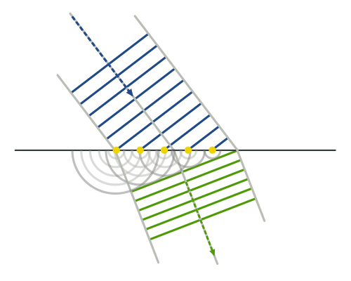
$500px-Refraction_-_Huygens-Fresnel_principle$

This comes from Wikipedia, as do the illustrations below. It does not only ‘explain’ diffraction gratings, but it also ‘explains’ what happens when light goes through a slit, cf. the second (animated) illustration.

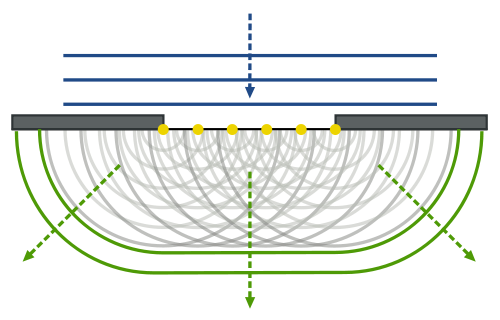
$500px-Refraction_on_an_aperture_-_Huygens-Fresnel_principle$

Now that, light being diffracted as it is going through a slit, is obviously much more mysterious than a diffraction grating – and, you’ll admit, a diffraction grating is already mysterious enough, because it’s rather strange that only certain points in the grating (i.e. the notches) would act as sources, isn’t it? Now, if that’s difficult to understand, it’s even more difficult to understand why an empty space, i.e. a slit, would act as a diffraction grating! However, because this post has become way too long already, we’ll leave this discussion for later.

Some content on this page was disabled on June 17, 2020 as a result of a DMCA takedown notice from Michael A. Gottlieb, Rudolf Pfeiffer, and The California Institute of Technology. You can learn more about the DMCA here:

https://en.support.wordpress.com/copyright-and-the-dmca/
Some content on this page was disabled on June 17, 2020 as a result of a DMCA takedown notice from Michael A. Gottlieb, Rudolf Pfeiffer, and The California Institute of Technology. You can learn more about the DMCA here:

https://en.support.wordpress.com/copyright-and-the-dmca/
Some content on this page was disabled on June 17, 2020 as a result of a DMCA takedown notice from Michael A. Gottlieb, Rudolf Pfeiffer, and The California Institute of Technology. You can learn more about the DMCA here:

https://en.support.wordpress.com/copyright-and-the-dmca/
Some content on this page was disabled on June 17, 2020 as a result of a DMCA takedown notice from Michael A. Gottlieb, Rudolf Pfeiffer, and The California Institute of Technology. You can learn more about the DMCA here:

https://en.support.wordpress.com/copyright-and-the-dmca/
Some content on this page was disabled on June 17, 2020 as a result of a DMCA takedown notice from Michael A. Gottlieb, Rudolf Pfeiffer, and The California Institute of Technology. You can learn more about the DMCA here:

https://en.support.wordpress.com/copyright-and-the-dmca/
Some content on this page was disabled on June 17, 2020 as a result of a DMCA takedown notice from Michael A. Gottlieb, Rudolf Pfeiffer, and The California Institute of Technology. You can learn more about the DMCA here:

https://en.support.wordpress.com/copyright-and-the-dmca/
Some content on this page was disabled on June 17, 2020 as a result of a DMCA takedown notice from Michael A. Gottlieb, Rudolf Pfeiffer, and The California Institute of Technology. You can learn more about the DMCA here:

https://en.support.wordpress.com/copyright-and-the-dmca/

Light and radiation

Pre-scriptum (dated 26 June 2020): Most of the relevant illustrations in this post were removed as a result of an attack by the dark force. In any case, you will probably prefer to read how my ideas on the theory of light and matter have evolved. If anything, posts like this document the historical path to them.

Original post:

Introduction: Scale Matters

One of the points which Richard Feynman, as a great physics teacher, does admirably well is to point out why scale matters. In fact, ‘old’ physics are not incorrect per se. It’s just that ‘new’ physics analyzes stuff at a much smaller scale.

For example, Snell’s Law, or Fermat’s Principle of Least Time, which were ‘discovered’ 500 years ago – and they are actually older, because they formalize something that the Greeks had already found out: refraction of light, as it travels from one medium (air, for example) into another (water, for example) – are still fine when studying focusing lenses and mirrors, i.e. geometrical optics. The dimensions of the analysis, or the equipment involved (i.e. the lenses or the mirrors), are huge as compared to the wavelength of the light and, hence, we can effectively look at light as a beam that travels from one point to another in a straight line, that bounces of a surface, or as a beam that gets refracted when it passes from one medium to another.

However, when we let the light pass through very narrow slits, it starts behaving like a wave. Geometrical optics does not help us, then, to understand its behavior: we will, effectively, analyze light as a wave-like thing at that scale, and analyze wave-like phenomena, such as interference, the Doppler effect and what have you. That level of analysis is referred to as the classical theory of electromagnetic radiation, and it’s what we’ll be introducing in this post.

The analysis of light as photons, i.e. as a bunch of ‘particles’ described by some kind of ‘wave function’ (which does not describe any real wave, but only some ‘probability amplitude’), is the third and final level of analysis, referred to as quantum mechanics or, to be more precise, as quantum electrodynamics (QED). [Note the terminology: quantum mechanics describes the behavior of matter particles, such as protons and electrons, while quantum electrodynamics (QED) describes the nature of photons, a force-carrying particle, and their interaction with matter particles.]

But so we’ll focus on the second level of analysis in this post.

Different mathematical approaches

One other thing which Feynman points out in his Lectures is that, even within a well-agreed level of analysis, there are different mathematical approaches to a problem. In fact, while, at any level of analysis, there’s (probably) only one fully mathematically correct analysis, approximate approaches may actually be easier to work with, not only because they actually allow us to solve a practical problem, but also because they help us to understand what’s going on.

Feynman’s treatment of electromagnetic radiation (Volume I, Chapters 28 to 34) is a case in point. While he notes that Maxwell’s field equations are actually the ones to be used, he writes them in a mathematical form that we can understand more easily, and then simplifies that mathematical form even further, in order to derive all that a sophomore student is supposed to know about electromagnetic radiation (EMR), which, of course, not only includes what we call light but also radio waves, radar waves, infrared waves and, on the other side of the spectrum, x-rays and gamma rays.

But let’s get down to business now.

The oscillating charge

Radiation is caused by some far-away electric charge (q) that’s moving in various directions in a non-uniform way, i.e. it is accelerating or decelerating, and perhaps reversing direction in the process. From our point of view (P), we draw a unit vector e_r’ in the direction of the charge. [If you want a drawing, there’s one further down.]

We write r’ (r prime), not r, because it is the retarded distance: when we look at the charge, we see where it was r’/c seconds ago: r’/c is indeed the time that’s needed for some influence to travel from the charge to the here and now, i.e. to P. So now we can write Coulomb’s Law:

E₁ = –qe_r’/4πe₀r’²

This formula can quickly be explained as follows:

The minus sign makes the direction of the force come out alright: like charges do not attract but repel, unlike gravitation. [Indeed, for gravitation, there’s only one ‘charge’, a mass, and masses always attract. Hence, for gravitation, the force law is that like charges attract, but so that’s not the case here.]
E and e_r’ and, hence, the electric force, are all directed along the line of sight.
The Coulomb force is proportional to the amount of charge, and the factor of proportionality is 1/4πe₀r’².
Finally, and most importantly in this context (study of EMR), the influence quickly diminishes with the distance: it varies inversely as the square of the distance (i.e. it varies as the inverse square).

Coulomb’s Law is not all that comes out of Maxwell’s field equations. Maxwell’s equations also cover electrodynamics. Fortunately, because we are, indeed, talking moving charges here, so electrostatics is only part of the picture and, in fact, the least important one in this case. 🙂 That’s why I wrote E₁, with as subscript, above – not E.

So we have a second term, and I’ll actually be introducing a third term in a minute or so. But let’s first look at the second term. I am not sure how Feynman derives it from Maxwell’s equations – I am sure I’ll see the light 🙂 when reading Volume II – but, from Maxwell’s equations, he does, somehow, derive the following, secondary, effect:

This is a term I struggled with in a first read, and I still do. As mentioned above, I need to read Feynman’s Volume II, I guess. But, while I still don’t understand the why, I now understand what this expression catches. The term between brackets is the Coulomb effect, which we mentioned above already, and the time derivative is the rate of change. We multiply that with the time delay (i.e. r’/c). So what’s going on? As Feynman writes it: “Nature seems to be attempting to guess what the field at the present time is going to be, by taking the rate of change and multiplying by the time that is delayed.”

OK. As said, I don’t really understand where this formula comes from but it makes sense, somehow. As for now, we just need to answer another question in order to understand what’s going on: in what direction is the Coulomb field changing?

It could be either: if the charge is moving along the direction of sight e_r’ won’t change but r’ will. However, if r’ does not change, then it’s e_r’ that changes direction, and that change will be perpendicular to the line of sight, or transverse (as opposed to radial), as Feynman puts it. Or, of course, it could be a combination of both. [Don’t worry too much if you’re not getting this: we will need this again in just a minute or so, and then I will also give you a drawing so you’ll see what I mean.]

The point is, these first two terms are actually not important because electromagnetic radiation is given by the third effect, which is written as:

Wow ! This looks even more complicated, doesn’t it? Let’s analyze it. The first thing to note is that there is no r’ or r’² in this equation. However, that’s an optical illusion of sorts, because r’ does matter when looking at that second-order derivative. How? Well… Let’s go step by step and first look at that second-order derivative. It’s the acceleration (or deceleration) of e_r’. Indeed, visualize e_r’ wiggling about, trying to follow the charge by pointing at where the charge was r’/c seconds ago. Let me help you here by, finally, inserting hat drawing I promised you.

This acceleration will have a transverse as well as a radial component: we can imagine the end of e_r’ (i.e. the point of the arrow) being on the surface of a unit sphere indeed. So as it wiggles about, the tip of the arrow moves back a bit from the tangential line. That’s the radial component of the acceleration. It’s easy to see that it’s quite small as compared to the transverse component, which is the component along the line that’s tangent to the surface (i.e. perpendicular to e_r’).

Now, we need to watch out: we are not talking displacement or velocity here but acceleration. Hence, even if the displacement of the charge is very small, and even if velocities would not be phenomenal either (i.e. non-relativistic), the acceleration involved can take on any value really. Hence, even with small displacements, we can have large accelerations, so the radial component is small relative to the transverse component only, not in an absolute sense.

That being said, it’s easy to see that both the transverse as well as the radial component depend on the distance r’ but in a different way. I won’t bother you with the geometrical proof (it’s not that obvious). Just accept that the radial component varies, more or less as the inverse square of the distance. Hence, we will simplify and say that we’re considering large distances r’ only – i.e. large in comparison to the length of the unit vector, which just means large in comparison to one (1) – and then it’s only the transverse component of a that matters, which we’ll denote by a_x.

However, if we drop that radial component, then we should drop E₁ as well, because the Coulomb effect will be very small as compared to the radiation effect (i.e. E₃). And, then, if we drop E₁, we can drop the ‘correction’ E₂ as well, of course. Indeed, that’s what Feynman does. He ends up with this third term only, which he terms the law of radiation:

So there we are. That’s all I wanted to introduce here. But let’s analyze it a bit more. Just to make sure we’re all getting it here.

The dipole radiator

All that simplification business above is tricky, you’ll say. First, why do we write t – r/c for the retarded time (t’)? It should be t – r’/c, no? You’re right. There’s another simplification here: we fix the delay time, assuming that the charge only moves very small distances at an effectively constant distance r. Think of some far-away antenna indeed.

Hmm… But then we have that 1/c² factor, so that should reduce the effect to zilch, isn’t it? And then… Hey! Wait a minute! Where does that r suddenly come from? Well, we’ve replaced d²e_r’/dt² by the lateral acceleration of the charge itself (i.e. its component perpendicular to the line of sight, denoted by a_x) divided by r. That’s just similar triangles.

Phew! That’s a lot of simplifications and/or approximations indeed. How do we know this law really works? And, if it does, for what distance? When is that 1/r part (i.e. E₃) so large as compared to the other two terms (E₁ and E₂) that the latter two don’t matter anymore? Well… That seems to depend on the wavelength of the radiation, but we haven’t introduced that concept yet. Let me conclude this first introduction by just noting this ‘law’ can easily be confirmed by experiment.

A so-called dipole oscillator or radiator can be constructed, as shown below: a generator drives electrons up and down in two wires (A and B). Why do we put the generator in the middle? That’s because we want a net effect: the radiation effect of the electrons in the wires connecting the generator with A and B will be neutral, because the electrons move right next to each other in opposite direction. With the generator in the middle, A and B form one antenna, which we’ll denote by G (for generator).

Now, another antenna can act as a receiver, and we can amplify the signal to hear it. That’s the D (for detector) shown below. Now, one of the consequences of the above ‘law’ for electromagnetic radiation is, obviously, that the strength of the received signal should become weaker as we turn the detector. The strongest signal should be when D is parallel to G. At point 2, there is a projection effect and, hence, the strength of the field should be less. Indeed, remember that the strength of the field is proportional to the acceleration of the charge projected perpendicular to the line of sight. Hence, at point 3, it should be zero, because the projection is zero.

Now, that’s what an experiment like this would indeed confirm. [I am tempted now to explain how a radio receiver works, but I will resist the temptation.]

I just need to make a last point here in order to make sure that we understand the formula above and – more importantly – that we can use in subsequent chapters without having to wonder where it comes from. The formula above implies that the direction of the field is at right angles to the line of sight. Now, if a charge is just accelerating up and down, in a motion of very small amplitude, i.e. like the motion in that antenna, then the magnitude (or strength let’s say) of the field will be given by the following formula:

θ, in this formula, is the angle between the axis of motion and the line of sight, as illustrated below:

So… That’s all we need to know for now. We’re done. As for now that is. This was quite technical, I guess, but I am afraid the next post will be even more technical. Sorry for that. I guess this is just a piece we need to get through.

Post scriptum:

You’ll remember that, with moving and accelerating charges, we should also have a magnetic field, usually denoted by B. That’s correct. If we have a changing electric field, then we will also have a magnetic field. There’s a formula for B:

B = –e_r’´E/c = –| e_r’||E|c^–1sin(e_r’, E)·n = –(E/c)·n

This is a vector cross-product. The angle between the unit vector e_r’ and E is π/2, so the sine is one. The vector n is the vector normal to both vectors as defined by the right-hand screw rule. [As for the minus sign, note that –a´b = b´a, so we could have reversed the vectors: the minus sign just reverses the direction of the normal vector.] In short, the magnetic field vector B is perpendicular to E, but its magnitude is tiny: E/c. That’s why Feynman neglects it, but we will come back on that in later posts.

Some content on this page was disabled on June 17, 2020 as a result of a DMCA takedown notice from Michael A. Gottlieb, Rudolf Pfeiffer, and The California Institute of Technology. You can learn more about the DMCA here:

https://en.support.wordpress.com/copyright-and-the-dmca/
Some content on this page was disabled on June 17, 2020 as a result of a DMCA takedown notice from Michael A. Gottlieb, Rudolf Pfeiffer, and The California Institute of Technology. You can learn more about the DMCA here:

https://en.support.wordpress.com/copyright-and-the-dmca/
Some content on this page was disabled on June 17, 2020 as a result of a DMCA takedown notice from Michael A. Gottlieb, Rudolf Pfeiffer, and The California Institute of Technology. You can learn more about the DMCA here:

https://en.support.wordpress.com/copyright-and-the-dmca/