Radiation and relativity

Pre-scriptum (dated 26 June 2020): Some of the relevant illustrations in this post were removed as a result of an attack by the dark force. Too bad, because I liked this post. In any case, despite the removal of the illustrations, you should be able to reconstruct the main story line.

Original post:

Now we are really going to do some very serious analysis: relativistic effects in radiation. Fasten your seat belts please.

The Doppler effect for physical waves traveling through a medium

In one of my post – I don’t remember which one – I wrote about the Doppler effect for sound waves, or any physical wave traveling through a medium. I also said it had nothing to do with relativity. What happens really is that the observer sort of catches up with wave or – the other way around: that he falls back – and, because the velocity of a wave in a medium is always the same (that also has nothing to do with relativity: it’s just a general principle that’s true – always), the frequency of the physical wave will appear to be different. [So that’s why a siren of an ambulance sounds different as it moves past you.] Wikipedia has an excellent article on that – so I’ll refer you to that – but so that article does not say anything – or nothing much – about the Doppler effect when electromagnetic radiation is involved. So that’s what we’ll talk about here. Before we do that, though, let me quickly jot down the formula for the Doppler effect for a physical wave traveling through a medium, so we are clear about the differences between the two ‘Doppler effects’:

In this formula, v_p is the propagation speed of the wave in the medium which – as mentioned above – depends on the medium. Now the source and the receiver will have a velocity with respect to the medium as well (positive or negative – depending on whether they’re moving in the same direction as the wave or not), and so that’s v_r (r for receiver) and v_s (s for source) respectively. So we’re adding speeds here to calculate some relative speed and then we take the ratio. Some people think that’s what relativity theory is all about. It’s not. Everything I’ve written so far is just Galilean relativity – so stuff that’s been known for a thousand years already, if not longer.

Relativity is weird: one aspect of it is length contraction – not often discussed – but the other thing is better known: there is no such thing as absolute time, so when we talk velocities, you need to specify according to whose time?

The Doppler effect for electromagnetic radiation

One thing that’s not relative – and which makes things look somewhat similar to what I wrote above – is that the speed of light is always equal to c. That was the startling fact that came out of Maxwell’s equations (startling because it is not consistent with Galilean relativity: it says that we cannot ‘catch up’ with a light wave!) around which Einstein build all of “new physics”, and so it’s something we use rather matter-of-factly in all that we’ll write below.

In all of the preceding posts about light, I wrote – more than once actually – that the movement of the oscillating charge (i.e. the source of the radiation) along the line of sight did not matter: the only thing that mattered was its acceleration in the xy-plane, which is perpendicular to our line of sight, which we’ll call the z-axis. Indeed, let me remind of you of the two equations defining electromagnetic radiation (see my post on light and radiation about a week ago):

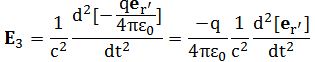
The first formula gives the electromagnetic effect that dominates in the so-called wave zone, i.e. a few wavelengths away from the source – because the Coulomb force varies as the inverse of the square of the distance r, unlike this ‘radiation’ effect, which varies inversely as the distance only (E ∝ 1/r), so it falls off much less rapidly.

Now, that general observation still holds when we’re considering an oscillating charge that is moving towards or away from us with some relativistic speed (i.e. a speed getting close enough to c to produce relativistic length contraction and time dilation effects) but, because of the fact that we need to consider local times, our formula for the retarded time is no longer correct.

Huh? Yes. The matter is quite complicated, and Feynman starts with jotting down the derivatives for the displacement in the x- and y-directions, but I think I’ll skip that. I’ll go for the geometrical picture straight away, which is given below. As said, it’s going to be difficult, but try to hang in here, because it’s necessary to understand the Doppler effect in a correct way (I myself have been fooled by quite a few nonsensical explanations of it in popular books) and, as a bonus, you also get to understand synchrotron radiation and other exciting stuff.

So what’s going on here? Well… Don’t look at the illustration above. We’ll come back at it. Let’s first build up the logic. We’ve got a charge moving vertically – from our point that is (the observer), but also moving in and out of us, i.e. in the z-direction. Indeed, note the arrow pointing to the observer: that’s us! So it could indeed be us looking at electrons going round and round and round – at phenomenal speeds – in a synchrotron indeed – but then one that’s been turned 90 degrees (probably easier for us to just lie down on the ground and look sideways). In any case, I hope you can imagine the situation. [If not, try again.] Now, if that charge was not moving at relativistic speeds (e.g. 0.94c, which is actually the number that Feynman uses for the graph above), then we would not have to worry about ‘our’ time t and the ‘local’ time τ. Huh? Local time? Yes.

We denote the time as measured in the reference frame of the moving charge as τ. Hence, as we are counting t = 1, 2, 3 etcetera, the electron is counting τ = 1, 2, 3 etcetera as it goes round and round and round. If the charge would not be moving at relativistic speeds, we’d do the standard thing and that’s to calculate the retarded acceleration of the charge a'(t) = a(t − r/c). [Remember that we used a prime to mark functions for which we should use a retarded argument and, yes, I know that the term ‘retarded’ sounds a bit funny, but that’s how it is. In any case, we’d have a'(t) = a(t − r/c) – so the prime vanishes as we put in the retarded argument.] Indeed, from the ‘law’ of radiation, we know that the field now and here is given by the acceleration of the charge at the retarded time, i.e. t – r/c. To sum it all up, we would, quite simply, relate t and τ as follows:

τ = t – r/c or, what amounts to the same, t = τ + r/c

So the effect that we see now, at time t, was produced at a distance r at time τ = t − r/c. That should make sense. [Again, if it doesn’t: read again. I can’t explain it in any other way.]

The crucial chain in this rather complicated chain of reasoning comes now. You’ll remember that one of the assumptions we used to derive our ‘law’ of radiation was that the assumption that “r is practically constant.” That does no longer hold. Indeed, that electron moving around in the synchrotron comes in and out at us at crazy speeds (0.94c is a bit more than 280,000 km per second), so r goes up and down too, and the relevant distance is not r but r + z(τ). This means the retardation effect is actually a bit larger: it’s not r/c but [r + z(τ)]/c = r/c + z(τ)/c. So we write:

τ = t – r/c – z(τ)/c or, what amounts to the same, t = τ + r/c + z(τ)/c

Hmm… You’ll say this is rather fishy business. Why would we use the actual distance and not the distance a while ago? Well… I’ll let you mull over that. We’ve got two points in space-time here and so they are separated both by distance as well as time. It makes sense to use the actual distance to calculate the actual separation in time, I’d say. If you’re not convinced, I can only refer you to those complicated derivations that Feynman briefly does before introducing this ‘easier’ geometric explanation. This brings us to the next point. We can measure time in seconds, but also in equivalent distance, i.e. light-seconds: the distance that light (remember: always at absolute speed c) travels in one second, i.e. approximately 299,792,458 meter. It’s just another ‘time unit’ to get used to.

Now that’s what’s being done above. To be sure, we get rid of the constant r/c, which is a constant indeed: that amounts to a shift of the origin by some constant (so we start counting earlier or later). In short, we have a new variable ‘t’ really that’s equal to t = τ + z(τ)/c. But we’re going to count time in meter (well – in units of c meter really), so we will just multiply this and we get:

ct = cτ + z(τ)

Why the different unit? Well… We’re talking relativistic speeds here, don’t we? And so the second is just an inappropriate unit. When we’re finished with this example, we’ll give you an even simpler example: a source just moving in on us, with an equally astronomical speed, so the functional shape of z(τ) will be some fraction of c (let’s say kc) times τ, so kcτ. So, to simplify things, just think of it as re-scaling the time axis in units that makes sense as compared to the speeds we are talking about.

Now we can finally analyze that graph on the right-hand side. If we would keep r fixed – so if we’d not care about the charge moving in and out of – the plot of x'(t) – i.e. the retarded position indeed – against ct would yield the sinusoidal graph plotted by the red numbers 1 to 13 here. In fact, instead of a sinusoidal graph, it resembles a normal distribution, but that’s just because we’re looking at one revolution only. In any case, the point to note is that – when everything is said and done – we need to calculate the retarded acceleration, so that’s the second derivative of x'(t). The animated illustration shows how that works: the second derivative (not the first) turns from positive to negative – and vice versa – at inflection points, when the curve goes from convex to concave, and vice versa. So, on the segment of that sinusoidal function marked by the red numbers, it’s positive at first (the slope of the tangent becomes steeper and steeper), then negative (cf. that tangent line turning from blue to green in the illustration below), and then it becomes positive again, as the negative slope becomes less negative at the second inflection point.

That should be straightforward. However, the actual x'(t) curve is the black curve with the cusp. A curve like that is called a hypocycloid. Let me reproduce it once again for ease of reference.

We relate x'(t) to ct (this is nothing but our new unit for t) by noting that ct = cτ + z(τ). Capito? It’s not easy to grasp: the instinct is to just equate t and τ and write x'(t) = x'(τ), but that would not be correct. No. We must measure in ‘our’ time and get a functional form for x’ as a function of t, not of τ. In fact, x'(t) − i.e. the retarded vertical position at time t – is not equal to x'(τ) but to x(τ), i.e. that’s the actual (instead of retarded) position at (local) time τ, and so that’s what the black graph above shows.

I admit it’s not easy. I myself am not getting it in an ‘intuitive’ way. But the logic is solid and leads us where it leads us. Perhaps it helps to think in terms of the curvature of this graph. In fact, we have to think in terms of curvature of this graph in order to understand what’s happening in terms of radiation. When the charge is moving away from us, i.e. during the first three ‘seconds’ (so that’s the 1-2-3 count), we see that the curvature is less than than what it would be – and also doesn’t change very much – if the displacement was given by the sinusoidal function, which means there’s very little radiation (because there’s little acceleration – negative or positive. However, as the charge moves towards us, we get that sharp cusp and, hence, we also get sharp curvature, which results in a sharp pulse of the electric field, rather than the regular – equally sinusoidal – amplitude we’d have if that electron was not moving in and out at us at relativistic speeds. In fact, that’s what synchrotron radiation is: we get these sharp pulses indeed. Feynman shows how they are measured – in very much detail – using a diffraction grating, but that would just be another diversion and so I’ll spare you of that.

Hmm… This has nothing to do with the Doppler effect, you’ll say. Well… Yes and no. The discussion above basically set the stage for that discussion. So let’s turn to that now. However, before I do that, I want to insert another graph for an oscillating charge moving in and out at us in some irregular way – rather than the nice circular route described above.

The Doppler effect

The illustration below is a similar diagram as the ones above – but looks much simpler. It shows what happens when an oscillating charge (which we assume to oscillate at its natural or resonant frequency ω₀) moves towards us at some relativistic speed v (whatever speed – fairly close to c, so the ratio v/c is substantial). Note that the movement is from A to B – and that the observer (we!) are, once again, at the left – and, hence, the distance traveled is AB = vτ. So what’s the impact on the frequency? That’s shown on the x'(t) graph on the right: the curvature of the sinusoidal motion is much sharper, which means that its angular frequency as we see or measure it (and we’ll denote that by ω₁) will be higher: if it’s a larger object emitting ‘white’ light (i.e. a mix of everything), then the light will not longer be ‘white’ but it will have shifted towards the violet spectrum. If it moves away from us, it will appear ‘more red’.

What’s the frequency change? Well… The z(τ) function is rather simple here: z(τ) = vτ. Let’s use f and f₀ for a moment, instead of the angular frequency ω and ω₀, as we know they only differ by the factor 2π (ω = 2π/T = 2π·f, with f = 1/T, i.e. the reciprocal of the period). Hence, in a given time Δτ, the number of oscillations will be f₀Δτ. These oscillations will be spread over a distance vΔτ, and the time needed to travel that distance is Δτ – of course! For the observer, however, the same number of oscillations now is compressed over a distance (c-v)Δτ. The time needed to travel that distance corresponds to a time interval Δt = (c − v)Δτ/c = (1 − v/c)Δτ. Now, hence, the frequency f will be equal to f₀Δτ (the number of oscillations) divided by Δt = (1 − v/c)Δτ. Hence, we get this relatively simple equation:

f = f₀/(1 − v/c) and ω = ω₀/(1 − v/c)

 Is that it? It’s not quite the same as the formula we had for the Doppler effect of physical waves traveling through a medium, but it’s simple enough indeed. And it also seems to use relative speed. Where’s the Lorentz factor? Why did we need all that complicated machinery?

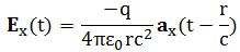
You are a smart ass ! You’re right. In fact, this is exactly the same formula: if we equal the speed of propagation with c, set the velocity of the receiver to zero, and substitute v (with a minus sign obviously) for the speed of the source, then we get what we get above:

The thing we need to add is that the natural frequency of an atomic oscillator is not the same as that measured when standing still: the time dilation effects kicks in. If w₀  is the ‘true’ natural frequency (so measured locally, so to say), then the modified natural frequency – as corrected for the time dilation effect – will be w₁ = w₀(1 – v²/c²)^1/2. Therefore, the grand final relativistic formula for the Doppler effect for electromagnetic radiation is:

You may feel cheated now: did you really have to suffer going through that story on the synchrotron radiation to get the formula above? I’d say: yes and no. No, because you could be happy with the Doppler formula alone. But, yes, because you don’t get the story about those sharp pulses just from the relativistic Doppler formula alone. So the final answer is: yes. I hope you felt it was worth the suffering 🙂

Some content on this page was disabled on June 17, 2020 as a result of a DMCA takedown notice from Michael A. Gottlieb, Rudolf Pfeiffer, and The California Institute of Technology. You can learn more about the DMCA here:

https://en.support.wordpress.com/copyright-and-the-dmca/
Some content on this page was disabled on June 17, 2020 as a result of a DMCA takedown notice from Michael A. Gottlieb, Rudolf Pfeiffer, and The California Institute of Technology. You can learn more about the DMCA here:

https://en.support.wordpress.com/copyright-and-the-dmca/