Euler’s formula revisited

Pre-scriptum (dated 26 June 2020): This post – part of a series of rather simple posts on elementary math and physics – did not suffer much from the attack by the dark force—which is good because I still like it. Enjoy !

Original post:

This post intends to take some of the magic out of Euler’s formula. In fact, I started doing that in my previous post but I think that, in this post, I’ve done a better job at organizing the chain of thought. [Just to make sure: with ‘Euler’s formula’, I mean e^ix = cos(x) + isin(x). Euler produced a lot of formulas, indeed, but this one is, for math, what E = mc² is for physics. :-)]

The grand idea is to start with an initial linear approximation for the value of the complex exponential e^is near s = 0 (to be precise, we’ll use the e^iε = 1 + iε formula) and then show how the ‘magic’ of i – through the i² = –1 factor – gives us the sine and cosine functions. What we are going to do, basically, is to construct the sine and cosine functions algebraically.

Let us, as a starting point – just to get us focused – graph (i) the real exponential function e^x, i.e. the blue graph, and (ii) the real and imaginary part of the complex exponential function e^ix = cos(x) + isin(x), i.e. the red and green graph—the cosine and sine function.   From these graphs, it’s clear that e^x and e^ix are two very different beasts.

1. e^x is just a real-valued function of x, so it ‘maps’ the real number x to some other real number y = e^x. That y value ‘rockets’ away, thereby demonstrating the power of exponential growth. There’s nothing really ‘special’ about e^x. Indeed, writing e^x instead of 10^x obviously looks better when you’re doing a blog on math or physics but, frankly, there’s no real reason to use that strange number e ≈ 2.718 when all you need is just a standard real exponential. In fact, if you’re a high school student and you want to attract attention with some paper involving something that grows or shrinks, I’d recommend the use of π^x. 🙂

2. e^ix is something that’s very different. It’s a complex-valued function of x and it’s not about exponential growth (though it obviously is about exponentiation, i.e. repeated multiplication): y = e^ix does not ‘explode’. On the contrary: y is just a periodic ‘thing’ with two components: a sine and a cosine. [Note that we could also change the base, to 10, for example: then we write 10^ix. We’d also get something periodic, but let’s not get lost before we even start.]

Two different beasts, indeed. How can the addition of one tiny symbol – the little i in e^ix – can make such big difference?

The two beasts have one thing in common: the value of the function near x = 0 can be approximated by the same linear formula:

In case you wonder where this comes from, it’s basically the definition of the derivative of a function, as illustrated below. 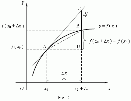This is nothing special. It’s a so-called first-order approximation of a function. The point to note is that we have a similar-looking formula for the complex-valued e^ix function. Indeed, its derivative is d(e^ix)/dx = ie^ix and when we evaluate that derivative at x = 0, then we get ie⁰ = i. So… Yes, the grand result is that we can effectively write:

e^iε ≈ 1 + iε for small ε

Of course, 1 + iε is also a different ‘beast’ than 1 +  ε. Indeed, 1 + ε is just a continuation of our usual walk along the real axis, but 1 +  iε points in a different direction (see below). This post will show you where it’s headed.

Let’s first work with e^x again, and think about a value for ε. We could take any value, of course, like 0.1 or some fraction 1/n. We’ll use a fraction—for reasons that will become clear in a moment. So the question now is: what value should we use for n in that 1/n fraction? Well… Because we are going to use this approximation as the initial value in a series of calculations—be patient: I’ll explain in a moment—we’d like to have a sufficiently small fraction, so our subsequent calculations based on that initial value are not too far off. But what’s sufficiently small? Is it 1/10, or 1/100,000, or 1/10¹⁰⁰? What gives us ‘good enough’ results? In fact, how do we define ‘good enough’?

Good question! In order to try to define what’s ‘good enough’, I’ll turn the whole thing on its head. In the table below, I calculate backwards from e¹ = e by taking successive square roots of e. Huh? What? Patience, please! Just go along with me for a while. First, I calculate e^1/2, so our fraction ε, which I’ll just write as  x, is equal to 1/2 here, so the approximation for e^1/2 is 1 + 1/2 = 1.5. That’s off. How much? Well… The actual value of e^1/2 is about 1.648721 (see the table below (or use a calculator or spreadsheet yourself): note that, because I copied the table from Excel, e^x is shown as e^x). Now, 1.648721 is 1.5 + 0.148721, so our approximation (1.5) is about 9% off (as compared to the actual value). Not all that much, but let’s see how we can improve. Let’s take the square root once again: (e^1/2)^1/2 = e^1/4, so x = 1/4. And then I do that again, so I get e^1/8, and so on and so on. All the way down to x = 1/1024 = 1/2¹⁰, so that’s ten iterations. Our approximation 1 + x (see the fifth/last column in the table below is then equal to 1 + 1/1024 = 1 + 0.0009765625, which we rounded to 1.000977 in the table.

The actual value of e^1/1024 is also about 1.000977, as you can see in the third column of the table. Not exactly, of course, but… Well… The accuracy of our approximation here is six digits behind the decimal point, so that’s equivalent to one part in a millionth. That’s not bad, but is it ‘good enough’? Hmm… Let’s think about it, but let’s first calculate some other things. The fourth column in the table above calculates the slope of that AB line in the illustration above: its value converges to one, as we would expect, because that’s the slope of the tangent line at x = 0. [So that’s the value of the derivative of e^x at x = 0. Just check it: de^x/dx = e^x, obviously, and e⁰ = 1.] Note that our 1 + x approximation also converges to 1—as it should!

So… Well… Let’s now just assume we’re happy with with that approximation that’s accurate to one part in a million, so let’s just continue to work with this fraction 1/1024 for x. Hence, we will write that e^1/1024 ≈ 1 + 1/1024 and now we will use that value also for the complex exponential. Huh? What? Why? Just hang in here for a while. Be patient. 🙂 So we’ll just add the i again and, using that e^iε ≈ 1 + iε expression, we write:

e^i/1024 ≈ 1 + i/1024

It’s quite obvious that 1 + i/1024 is a complex number: its real part is 1, and its imaginary part is 1/1024 = 0.0009765625.

Let’s now work our way up again by using that complex number 1 + i/1024 = 1 + i·0.0009765625 to calculate e^i/512, e^i/256, e^i/128 etcetera. All the way back up to x = 1, i.e. eⁱ. I’ll just use a different symbol for x: in the table below, I’ll substitute x for s because I’ll refer to the real part of our complex numbers as ‘x’ from time to time (even if I write a and b in the table below), and so I can’t use the symbol x to denote the fraction. [I could have started with s, but then… Well… Real numbers are usually denoted by x, and so it was easier to start that way.] In any case…

The thing to note is how I calculate those values e^i/512, e^i/256, e^i/128 etcetera. I am doing it by squaring, i.e. I just multiply the (complex) number by itself. To be very explicit, note that e^i/512 = (e^i/1024)² = e^i·2/1024 = (e^i/1024)(e^i/1024). So all that I am doing in the table below is multiply the complex number that I have with itself, and then I have a new result, and then I square that once again, and then again, and again, and again etcetera. In other words, when going back up, I am just taking the square of a (complex) number. Of course, you know how to multiply a number with itself but, because we’re talking complex numbers here, we should actually write it out:

(a + i·b)² = a² – b² + i·2ab = a² – b² + 2abi

[It would be good to always separate the imaginary unit i from real numbers like a, b, or ab, but then I am lazy and so I hope you’ll always recognize that i is the imaginary unit.] In any case… When we’re going back up (by squaring), the real part of the next number (i.e. the ‘x’ in x + iy) is a² – b² and the complex part (the ‘y’) is 2abi. So that’s what’s shown below—in the fourth and fifth column, that is.

Look at what happens. The x goes to zero and then becomes negative, and the y increases to one. Now, we went down from e^1/n = e¹ = e^1/1 to e^1/n = e^1/1024, but we could have started with e², or e^4/n, or whatever. Hence, I should actually continue the calculations above so you can see what happens when s goes to 2, and then to 3, and then to 4, and so on and so on. What you’d see is that the value of the real and imaginary part of this complex exponential goes up and down between –1 and +1. You’d see both are periodic functions, like the sine and cosine functions, which I added in the last two columns of the table above. Now compare those a and b values (i.e. the second and third column) with the cosine and sine values (i.e. the last two columns). […] Do you see it? Do you see how close they are? Only a few parts in a million, indeed.

You need to let this sink it for a while. And I’d recommend you make a spreadsheet yourself, so you really ‘get’ what’s going on here. It’s all there is to the so-called ‘magic’ of Euler’s formula. That simple (a + ib)² = a² – b² + 2abi formula shows us why (and how) the real and imaginary part oscillate between –1 and +1, just like the cosine and sine function. In fact, the values are so close that it’s easy to understand what follows. They are the same—in the limit, of course. 

Indeed, these values a² – b² and 2ab, i.e. the real and imaginary part of the next complex number in our series, are what Feynman refers to as the algebraic cosine and sine functions, because we calculate them as (a + ib)² = a² – b² + 2abi. These algebraic cosine and sine values are close to the real cosine and sine values, especially for small fractions s. Of course, there is a discrepancy becomes – when everything is said and done – we do carry a little error with us from the start, because we stopped at 1/n = 1/1024, before going back up.

There’s actually a much more obvious way to appreciate the error: we know that e^1/1024 should be some point on the unit circle itself. Therefore, we should not equate a with 1 if we have some value b > 0. Or – what amounts to saying the same – if if b is slightly bigger than 0, then a should be slightly smaller than 1. So the e^iε ≈ 1 + iε is an approximation only. It cannot be exact for positive values of ε. It’s only exact when ε = 0.

So we’re off—but not far off as you can see. In addition, you should note that the error becomes bigger and bigger for larger s. For example, in the line for s = 1, we calculated the values of the algebraic cosine and sine for s = 2 (see the a^2 – b^2 and 2ab column) as –0.416553 and 0.910186, but the actual values are cos(2) = –0.416146 and sin(2) = 0.909297, which shows our algebraic cosine and sine function is gradually losing accuracy indeed (we’re off like one part in a thousand here, instead of one part in a million). That’s what we’d expect, of course, as we’re multiplying the errors as we move ‘back up’.

The graph below plots the values of the table.

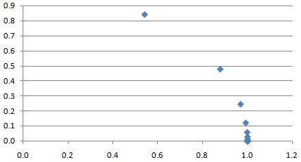
This graph also shows that, as we’re doubling our ratio r all the time, the data points are being spaced out more and more. This ‘spacing out’ gets a lot worse when further increasing s: from s = 1 (that’s the ‘highest’ point in the graph above), we’d go to s = 2, and then to s = 4, s = 8, etcetera. Now, these values are not shown above but you can imagine where they are: for s = 2, we’re somewhere in the second quadrant, for s = 4, we’re in the third, etcetera. So that does not make for a smooth graph. We need points in-between. So let’s ‘fix’ this problem by taking just one value for s out of the table (s = 1/4, for example) and we’ll continue to use that value as a multiplier.

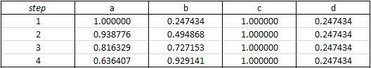
That’s what’s done in the table below. It looks somewhat daunting at first but it’s simple really. First, we multiply the value we got for e^1/4 with itself once again, so that gives us a real and an imaginary part for e^1/8 (we had that already in the table above and you can check: we get the same here). We then take that value (i.e. e^1/8) not to multiply it with itself but with e^1/4 once again. Of course, because the complex numbers are not the same, we cannot use the (a + ib)² = a² – b² + 2abi rule any more. We must now use the more general rule for multiplying different complex numbers: (a + ib)(c + id) = (ac – bd) + i(ad + bc). So that’s why I have an a, b, c and d column in this table: a and b are the components of the first number, and c and d of the second (i.e. e^1/4 = 0.969031 + 0.247434i)

In the table above, I let s range from zero (0) to seven (7) in steps of 0.25 (= 1/4). Once again, I’ve added the real cosine and sine values for these angles (they are, of course, expressed in radians), because that’s what s is here: an angle, aka as the phase of the complex number. So you can compare.

The table confirms, once again, that we’re slowly losing accuracy (we’re now 3 to 4 parts in a thousand off), but it is very slowly only indeed: we’d need to do many ‘loops’ around the center before we could actually see the difference on a graph. Hey! Let’s do a graph. [Excel is such a great tool, isn’t it?] Here we are: the thick black line describing a circle on the graph below connects the actual cosine and sine values associated with an angle of 1/4, 1/2, 3/8 etcetera, all the way up to 7 (7 is about 2.3π, so we’re some 40 degrees past our original point after the ‘loop’), while the little ‘+‘ marks are the data points for the algebraic cosine and sine. They match perfectly because our eye cannot see the little discrepancy.

So… That’s it. End of story.

What?

Yes. That’s it. End of story. I’ve done what I promised to do. I constructed the sine and cosine functions algebraically. No compass. 🙂 Just plain arithmetic, including one extra rule only: i² = –1. That’s it.

So I hope I succeeded. The goal was to take some of the magic out of Euler’s formula by showing how that e^iε = 1 + iε approximation and the definition of i² = –1 gives us the cosine and sine function itself as we move around the unit circle starting from the unity point on the real axis, as shown in that little graph:

Of course, the ε we were working with was much smaller than the size of the arrow suggests (it was equal to 1/1024 ≈ 0.000977 to be precise) but that’s just to show how differentials work. 🙂 Pretty good, isn’t it? 🙂

Post scriptum:

I. If anything, all this post did was to demonstrate multiplication of complex numbers. Indeed, when everything is said and done, exponentiation is repeated multiplication–both for real as well as for complex exponents. The only difference is–well… Complex exponents give us these oscillating things, because a complex exponent effectively throws a sine and cosine function in.

Now, we can do all kinds of things with that. In this post, we constructed a circle without a compass. Now, that’s not as good as squaring the circle 🙂 but, still, it would have awed Pythagoras. Below, I construct a spiral doing the same kind of math: I start off with a complex number again but now it’s somewhat more off the unit circle (1 + 0.247434i). In fact, I took the same sine value as the one we had for e^i/4 but I replaced the cosine value (0.969031) with 1 exactly). In other words, my ε is a lot bigger here.

Then I multiply that complex number 1 + 0.247434i with itself to get the next number (0.938776 + 0.494868i), and then I multiply that result once again with my first number (1 + 0.247434i), just like we did when we were constructing the circle. And then it goes on and on and on. So the only difference is the initial value: that’s a bit more off the unit circle. [When we constructed the circle, our initial value was also a bit off but much less. Here we go for a much larger difference.]

So you can see what happens: multiplying complex numbers amounts to adding angles and multiplying magnitudes: αe^iβ·γe^iδ = αγe^i(β+δ) =|αe^iβ|·|γe^iδ|e^i(β+δ)| = |α||γ|e^i(β+δ). So, because we started off with a complex number with magnitude slightly bigger than 1 (you calculate it using Pythagoras’ theorem: it’s 1.03, more or less, which is 3% off, as opposed less than one part in a million for the 1 + 0.000977i number), the next point is, of course, slightly off the unit circle too, and some more than 3% actually. And so that goes on and on and on and the ‘some more’ becomes bigger and bigger in the process.

Constructing a graph like this one is like doing the kind of silly stuff I did when programming little games with our Commodore 64 in the 1980s, so I shouldn’t dwell too much on this. In fact, now that I think of it: I should have started near –i, then my spiral would have resembled an e. 🙂 And, yes – for family reading this – this is also like the favorite hobby of our dad: calculating a better value for π. 🙂

However… The only thing I should note, perhaps, is that this kind of iterative process resembles – to some extent – the kind of process that iterative function systems (IFSs) use to create fractals. So… Well… It’s just nice, I guess. [OK. That’s just an excuse. Sorry.]

II. The other thing that I demonstrated in this post may seem to be trivial but I’ll emphasize it here because it helped me (not sure about you though) to understand the essence of real exponentials much better than I did before. So, what is it?

Well… It’s that rather remarkable fact that calculating (real) irrational powers amounts to doing some infinite iteration. What do I mean with that?

Well… Remember that we kept on taking the square root of e, so we calculated e^1/2, and then (e^1/2)^1/2 = e^1/4, and then (e^1/4)^1/2 = e^1/8, and then we went on: e^1/16, e^1/32, e^1/64, all the way down to e^1/1024, where we stopped. That was 10 iterations only. However, it was clear we could go on and on and on, to find that limit we know so well: e^1/Δ tends to 1 (not to zero (0), and not to e either!) for Δ → ∞.

Now, e = e¹ is an exponential itself and so we can switch to another base, base-10 for example, using the general a^s = (b^k)^s = b^ks = b^t formula, with k = log_b(a). Let’s do base-10: we get e¹ = [10^log₁₀(e)]¹ =  10^{0.434294…etcetera}. Now, because e is an irrational number, log₁₀(e) is irrational too, so we indeed have an infinite number of decimals behind the decimal point in 0.434294…etcetera. In fact, e is not only irrational but transcendental: we can’t calculate it algebraically, i.e. as the root of some polynomial with rational coefficients. Most irrational numbers are like that, by the way, so don’t think that being ‘transcendental’ is very special. In any case… That’s a finer point that doesn’t matter much here. You get the idea, I hope. It’s the following:

1. When we have a rational power a^m/n , it helps to think of it as a product of m factors a^1/n (and surely if we would want to calculate a^m/n without using a calculator, which, I admit, is not very fashionable anymore and so nobody ever does that: too bad, because the manual work involved does help to better understand things). Let’s write it down: a^m/n = a^m·(1/n) =(a^1/n)^m = a^1/n·a^1/n·a^1/n·a^1/n =·… (m times). That’s simple indeed: exponentiation is repeated multiplication. [Of course, if m is negative, then we just write a^m/n as 1/(a^m/n), but so that doesn’t change the general idea of exponentiation.]
2. However, it is much more difficult to see why, and how, exponentiation with irrational powers amounts to repeated multiplication too. The rather lengthy exposé above shows… Well, perhaps not why, but surely how. [And in math, if we can show how, that usually amounts to showing why also, isn’t it? :-)] Indeed, when we think of a^r (i.e. an irrational power of some (real) number a), we can think of it as a product of an infinite number of factors a^r/Δ. Indeed, we can write a^r as:

a^r = a^{r(1/Δ + 1/Δ + 1/Δ + 1/Δ +…)} = a^r/Δ·a^r/Δ·a^r/Δ·a^r/Δ…

Not convinced? Let’s work an example: 10^π = [e^ln10]^π = [e^ln10]^π = e^ln10·π = e^ln10·π = e^7.233784… Of course, if you take your calculator, you’ll find something like 1385.455731, both for 10^π  and e^7.233784 (hopefully!), but so that’s not the point here. We’ve shown that e is an infinite product e^1/Δ·e^1/Δ·e^1/Δ·e^1/Δ·… =e^{(1/Δ+1/Δ+1/Δ+1/Δ+…)} = e^Δ/Δ with Δ some infinitely large (but integer) number. In our example, we stopped the calculation at Δ = 1024, but you see the logic: we could have gone on forever. Therefore, we can write e^7.233784… as

e^7.233784… = e^{7.233784…(1/Δ+1/Δ+1/Δ+1/Δ+…)} = e^{7.233784…/Δ}·e^{7.233784…/Δ}·e^{7.233784…/Δ}…

Still not convinced? Let’s revert back to base 10. We can write the factors e^{7.233784…/Δ} as e^{(ln10·π)/Δ} = [e^ln10]^π/Δ = 10^π/Δ. So our original power 10^π is equal to: 10^π = 10^π/Δ·10^π/Δ·10^π/Δ·10^π/Δ·10^π/Δ·10^π/Δ… = 10^π(Δ/Δ), and of course, 10^1/Δ also tends to 1 as Δ goes to infinity (not to zero, and not to 10 either). 🙂 So, yes, we can do this for any real number a and for any r really.

Again, this may look very trivial to the trained mathematical eye but, as a novice in Mathematical Wonderland, I felt I had to go through this to truly understand irrational powers. So it may or may not help you, depending on where you are in MW.

[Proving that the limit for Δ/Δ goes to 1 as Δ goes to ∞ should not be necessary, I hope? 🙂 But, just in case you wonder how the formula for rational and irrational powers could possibly be related, we can just write a^m/n = a^{(m/n)(1/Δ + 1/Δ + 1/Δ + 1/Δ +…)} = a^m/nΔ·a^m/nΔ·a^m/nΔ·a^m/nΔ·…= (a^{1/Δ + 1/Δ + 1/Δ + 1/Δ +…})^m/n = a^m/n, as we would expect. :-)]

III. So how does that a^r = a^r/Δ·a^r/Δ·a^r/Δ·a^r/Δ… formula work for complex exponentials? We just add the i, so we write a^ir but we know what effect that has: we have a different beast now. A complex-valued function of r, or… Well… If we keep the exponent fixed, then it’s a complex-valued function of a! Indeed, do remember we have a choice here (and two inverse functions as well!).

However, note that we can write a^ir in two slightly different ways. We have two interpretations here really:

A. The first interpretation is the easiest one: we write a^ir as a^ir =  (a^r)ⁱ = (a^{r/Δ + r/Δ + r/Δ + r/Δ +…})ⁱ.

So we have a real power here, a^r, and so that’s some real number, and then we raise it to the power i to create that new beast: a complex-valued function with two components, one imaginary and one real. And then we know how to relate these to the sine and cosine function: we just change the base to e and then we’re done.

In fact, now that we’re here, let’s go all the way and do it. As mentioned in my previous post  – it follows out of that a^s = (e^k)^s = e^ks = e^t formula, with k = ln(a) – the only effect of a change of base is a change of scale of the horizontal axis: the graph of a^s is fully identical to the graph of e^t indeed: we just we need to substitute s by t = ks = ln(a)·s. That’s all. So we actually have our ‘Euler formula for a^is here. For example, for base 10, we have 10^is = cos[ln(a)·s] + isin[ln(a)·s].

But let’s not get lost in the nitty-gritty here. The idea here is that we let i ‘act’ on a^r, so to say. And then, of course, we can write a^r as we want, but that doesn’t change the essence of what we’re dealing with.

B. The second interpretation is somewhat more tricky: we write a^ir as a^ir = a^ir/Δ·a^ir/Δ·a^ir/Δ·a^ir/Δ·…

So that’s a product of an (infinite) number of complex factors a^ir/Δ. Now, that is a very different interpretation than the one above, even if the mathematical result when putting real numbers in for a and r will – obviously – have to be the same. If the result is the same, then what am I saying really? Well… Nothing much, I guess. Just that the interpretation of an exponentiation as repeated multiplication makes sense for complex exponentials as well:

• For rational r, we’ll have a finite number of complex factors: a^im/n = a^i/n·a^i/n·a^i/n·a^i/n·… (m times).
• For irrational r, we’ll have an infinite number of complex factors a^ir = a^ir/Δ·a^ir/Δ·a^ir/Δ·a^ir/Δ… etcetera.

So the difference with the first interpretation is that, instead of looking at a^ir as a real number a^r that’s being raised to the complex power i, we’re looking at a^ir as a complex number aⁱ that’s being raised to the real power r. As said, the mathematical result when putting real numbers in for a and r will – obviously – have to be the same. [Otherwise we’d be in serious trouble of course: math is math. We can’t have the same thing being associated with two different results.] But, as said, we can effectively interpret a^ir in two ways.

[…]

What I am doing here, of course, is contemplating all kinds of mathematical operations here – including exponentiation – on the complex space, rather on the real space. So the first step is to raise a complex number to a real power (as opposed to raising a real number to a complex power). The next step will be to raise a complex number to a complex power. So then we’re talking complex-valued functions of complex variables.

Now, that’s what complex analysis is all about, and I’ve written very extensively about that in my October-November 2013 post. So I would encourage you to re-read those, now that you’ve got, hopefully, a bit more of an ‘intuitive’ understanding of complex numbers with the background given in this and my previous post.

Complex analysis involves mapping (i.e. mapping from one complex space to another) and that, in turn, involves the concept of so-called analytic and/or holomorphic functions. Understanding those advanced concepts is, in turn, essential to understanding the kind of things that Penrose is writing about in Chapter 9 to 12 of his Road to Reality. […] I’ll probably re-visit these chapters myself in the coming weeks, as I realize I might understand them somewhat better now. If I could get through these, I’d be at page 250 or so, so that’s only one quarter of the total volume. Just an indication of how long that Road to Reality really is. 🙂

And then I am still not sure if it really leads to ‘reality’ because, when everything is said and done, those new theories (supersymmetry, M-theory, or string theory in general) are quite speculative, aren’t they? 🙂