Modes in classical and in quantum physics

Pre-scriptum (dated 26 June 2020): These posts on elementary math and physics have not suffered much from the attack by the dark force—which is good because I still like them. While my views on the true nature of light, matter and the force or forces that act on them have evolved significantly as part of my explorations of a more realist (classical) explanation of quantum mechanics, I think most (if not all) of the analysis in this post remains valid and fun to read. In fact, I find the simplest stuff is often the best. 🙂

Original post:

Basics

Waves are peculiar: there is one single waveform, i.e. one motion only, but that motion can always be analyzed as the sum of the motions of all the different wave modes, combined with the appropriate amplitudes and phases. Saying the same thing using different words: we can always analyze the wave function as the sum of a (possibly infinite) number of components, i.e. a so-called Fourier series:

The f(t) function can be any wave, but the simple examples in physics textbooks usually involve a string or, in two dimensions, some vibrating membrane, and I’ll stick to those examples too in this post. Feynman calls the Fourier components harmonic functions, or harmonics tout court, but the term ‘harmonic’ refers to so many different things in math that it may be better not to use it in this context. The component waves are sinusoidal functions, so sinusoidals might be a better term but it’s not in use, because a more general analysis will use complex exponentials, rather than sines and/or cosines. Complex exponentials (e.g. 10^ix) are periodic functions too, so they are totally unlike real exponential functions (e.g. (e.g. 10^x). Hence, Feynman also uses the term ‘exponentials’. At some point, he also writes that the pattern of motion (of a mode) varies ‘exponentially’ but, of course, he’s thinking of complex exponentials, and, therefore, we should substitute ‘exponentially’ for ‘sinusoidally’ when talking real-valued wave functions.

[…] I know. I am already getting into the weeds here. As I am a bit off-track anyway now, let me make another remark here. You may think that we have two types of sinusoidals, or two types of functions, in that Fourier decomposition: sines and cosines. You should not think of it that way: the sine and cosine function are essentially the same. I know your old math teacher in high school never told you that, but it’s true. They both come with the same circle (yes, I know that’s ridiculous statement but I don’t know how to phrase it otherwise): the difference between a sine and a cosines is just a phase shift: cos(ωt) = sin(ωt + π/2) and, conversely, sin(ωt) = cos(ωt − π/2). If the starting phases of all of the component waves would be the same, we’d have a Fourier decomposition involving cosines only, or sines only—whatever you prefer. Indeed, because they’re the same function except for that phase shift (π/2), we can always go from one to the other by shifting our origin of space (x) and/or time (t). However, we cannot assume that all of the component waves have the same starting phase and, therefore, we should write each component as cos(n·ωt + Φ_n), or a sine with a similar argument. Now, you’ll remember – because your math teacher in high school told you that at least 🙂 – that there’s a formula for the cosine (and sine) of the sum of two angles: we can write cos(n·ωt + Φ_n) as cos(n·ωt + Φ_n) = [cos(Φ_n)·cos(n·ωt) – sin(Φ_n)·sin(n·ωt)]. Substituting cos(Φ_n) and – sin(Φ_n) for a_n and b_n respectively gives us the a_n·cos(n·ωt) + b_n·sin(n·ωt) expressions above. In addition, the component waves may not only differ in phase, but also in amplitude, and, hence, the a_n and b_n coefficients do more than only capturing the phase differences. But let me get back on the track. 🙂

Those sinusoidals have a weird existence: they are not there, physically—or so it seems. Indeed, there is one waveform only, i.e. one motion only—and, if it’s any real wave, it’s most likely to be non-sinusoidal. At the same time, I noted, in my previous post, that, if you pluck a string or play a chord on your guitar, some string you did not pluck may still pick up one or more of its harmonics (i.e. one or more of its overtones) and, hence, start to vibrate too! It’s the resonance phenomenon. If you have a grand piano, it’s even more obvious: if you’d press the C4 key on a piano, a small hammer will strike the C4 string and it will vibrate—but the C5 string (one octave higher) will also vibrate, although nothing touched it—except for the air transmitting the sound wave (including the harmonics causing the resonance) from the C4 string, of course! So the component waves are there and, at the same time, they’re not. Whatever they are, they are more than mathematical forms: the so-called superposition principle (on which the Fourier analysis is based) is grounded in reality: it’s because we can add forces. I know that sounds extremely obvious – or ridiculous, you might say 🙂 – but it is actually not so obvious. […] I am tempted to write something about conservative forces here but… Well… I need to move on.

Let me show that diagram of the first seven harmonics of an ideal string once again. All of them, and the higher ones too, would be in our wave function. Hence, assuming there’s no phase difference between the harmonics, we’d write:

f(t) = sin(ωt) + sin(2ωt) + sin(3ωt) + … + sin(nωt) + …

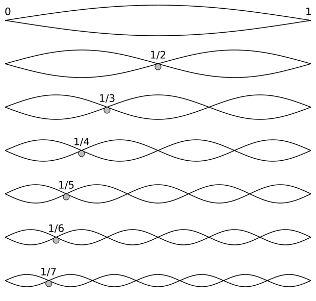
The frequencies of the various modes of our ideal string are all simple multiples of the fundamental frequency ω, as evidenced from the argument in our sine functions (ω, 2ω, 3ω, etcetera). Conversely, the respective wavelengths are λ, λ/2, λ/3, etcetera. [Remember: the speed of the wave is fixed, and frequency and wavelength are inversely proportional: c = λ·f = λ/T = λ·(ω/2π).] So, yes, these frequencies and wavelengths can all be related to each other in terms of equally simple harmonic ratios: 1:2, 2:3, 3:5, 4:5 etcetera. I explained in my previous posts why that does not imply that the musical notes themselves are related in such way: the musical scale is logarithmic. So I won’t repeat myself. All of the above is just an introduction to the more serious stuff, which I’ll talk about now.

Modes in two dimensions

An analysis of waves in two dimensions is often done assuming some drum membrane. The Great Teacher played drums, as you can see from his picture in his Lectures, and there are also videos of him performing on YouTube. So that’s why the drum is used almost all textbooks now. 🙂

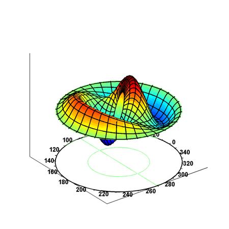
The illustration of one of the normal modes of a circular membrane comes from the Wikipedia article on modes. There are many other normal modes – some of them with a simpler shape, but some of them more complicated too – but this is a nice one as it also illustrates the concept of a nodal line, which is closely related to the concept of a mode. Huh? Yes. The modes of a one-dimensional string have nodes, i.e. points where the displacement is always zero. Indeed, as you can see from the illustration above (not below), the first overtone has one node, the second two, etcetera. So the equivalent of a node in two dimensions is a nodal line: for the mode shown below, we have one bisecting the disc and then another one—a circle about halfway between the edge and center. The third nodal line is the edge itself, obviously. [The author of the Wikipedia article nodes that the animation isn’t perfect, because the nodal line and the nodal circle halfway the edge and the center both move a little bit. In any case, it’s pretty good, I think. I should also learn how to make animations like that. :-)]

What’s a mode?

How do we find these modes? And how are they defined really? To explain that, I have to briefly return to the one-dimensional example. The key to solving the problem (i.e. finding the modes, and defining their characteristics) is the following fact: when a wave reaches the clamped end of a string, it will be reflected with a change in sign, as illustrated below: we’ve got that F(x+ct) wave coming in, and then it goes back indeed, but with the sign reversed.

It’s a complicated illustration because it also shows some hypothetical wave coming from the other side, where there is no string to vibrate. That hypothetical wave is the same wave, but travelling in the other direction and with the sign reversed (–F). So what’s that all about? Well… I never gave any general solution for a waveform traveling up and down a string: I just said the waveform was traveling up and down the string (now that is obvious: just look at that diagram with the seven first harmonics once again, and think about how that oscillation goes up and down with time), but so I did not really give any general solution for them (the sine and cosine functions are specific solutions). So what is the general solution?

Let’s first assume the string is not held anywhere, so that we have an infinite string along which waves can travel in either direction. In fact, the most general functional form to capture the fact that a waveform can travel in any direction is to write the displacement y as the sum of two functions: one wave traveling one way (which we’ll denote by F), and the other wave (which we’ll denote by G) traveling the other way. From the illustration above, it’s obvious that the F wave is traveling towards the negative x-direction and, hence, its argument will be x + ct. Conversely, the G wave travels in the positive x-direction, so its argument is x – ct. So we write:

y = F(x + ct) + G(x – ct)

[I’ve explained this thing about directions and why the argument in a wavefunction (x ± ct) is what it is before. You should look it up in case you don’t understand. As for the c in this equation, that’s the wave velocity once more, which is constant and which depends, as always, on the medium, so that’s the material and the diameter and the tension and whatever of the string.]

So… We know that the string is actually not infinite, but that it’s fixed to some ‘infinitely solid wall’ (as Feynman puts it). Hence, y is equal to zero there: y = 0. Now let’s choose the origin of our x-axis at the fixed end so as to simplify the analysis. Hence, where y is zero, x is also zero. Now, at x = 0, our general solution above for the infinite string becomes  y = F(ct) + G(−ct) = 0, for all values of t. Of course, that means G(−ct) must be equal to –F(ct). Now, that equality is there for all values of t. So it’s there for all values of ct and −ct. In short, that equality is valid for whatever value of the argument of G and –F. As Feynman puts it: “G of anything must be –F of minus that same thing.” Now, the ‘anything’ in G is its argument: x – ct, so ‘minus that same thing’ is –(x – ct) = −x + ct. Therefore, our equation becomes:

y = F(x + ct) − F(−x + ct)

So that’s what’s depicted in the diagram above: the F(x + ct) wave ‘vanishes’ behind the wall as the − F(−x + ct) wave comes out of it. Conversely, the − F(−x + ct) is hypothetical indeed until it reaches the origin, after which it becomes the real wave. Their sum is only relevant near the origin x = 0, and on the positive side only (on the negative side of the x-axis, the F and G functions are both hypothetical). [I know, it’s not easy to follow, but textbooks are really short on this—which is why I am writing my blog: I want to help you ‘get’ it.]

Now, the results above are valid for any wave, periodic or not. Let’s now confine the analysis to periodic waves only. In fact, we’ll limit the analysis to sinusoidal wavefunctions only. So that should be easy. Yes. Too easy. I agree. 🙂

So let’s make things difficult again by introducing the complex exponential notation, so that’s Euler’s formula: e^iθ = cosθ + isinθ, with i the imaginary unit, and isinθ the imaginary component of our wave. So the only thing that is real, is cosθ.

What the heck? Just bear with me. It’s good to make the analysis somewhat more general, especially because we’ll be talking about the relevance of all of this to quantum physics, and in quantum physics the waves are complex-valued indeed! So let’s get on with it. To use Euler’s formula, we need to substitute x + ct for the phase of the wave, so that involves the angular frequency and the wavenumber. Let me just write it down:

F(x + ct) = e^iω(t+x/c) and F(−x + ct) = e^iω(t−x/c)

Huh? Yeah. Sorry. I’ll resist the temptation to go off-track here, because I really shouldn’t be copying what I wrote in other posts. Most of what I write above is really those simple relations: c = λ·f = ω/k, with k, i.e. the wavenumber, being defined as k = 2π/λ. For details, go to one of my others posts indeed, in which I explain how that works in very much detail: just click on the link here, and scroll down to the section on the phase of a wave, in which I explain why the phase of wave is equal to θ = ωt–kx = ω(t–x/c). And, yes, I know: the thing with the wave directions and the signs is quite tricky. Just remember: for a wave traveling in the positive x-direction, the signs in front of x and t are each other’s opposite but, if the wave’s traveling in the negative y-direction, they are the same. As mentioned, all the rest is usually a matter of shifting the phase, which amounts to shifting the origin of either the x- or the t-axis. I need to move on. Using the exponential notation for our sinusoidal wave, y = F(x + ct) − F(−x + ct) becomes:

y = e^iω(t+x/c) − e^iω(t−x/c)

I can hear you sigh again: Now what’s that for? What can we do with this? Just continue to bear with me for a while longer. Let’s factor the e^iωt term out. [Why? Patience, please!] So we write:

y = e^iωt [e^iωx/c) − e^−iωx/c)]

Now, you can just use Euler’s formula again to double-check that e^iθ − e^−θ = 2isinθ. [To get that result, you should remember that cos(−θ) = cosθ, but sin(−θ) = −sin(θ).] So we get:

y = e^iωt [e^iωx/c) − e^−iωx/c)] = 2ie^iωtsin(ωx/c)

Now, we’re only interested in the real component of this amplitude of course – but that’s only we’re in the classical world here, not in the real world, which is quantum-mechanical and, hence, involves the imaginary stuff also 🙂 – so we should write this out using Euler’s formula again to convert the exponential to sinusoidals again. Hence, remembering that i² = −1, we get:

y = 2ie^iωtsin(ωx/c) = 2icos(ωt)·sin(ωx/c) – 2sin(ωt)·sin(ωx/c)

!?!

OK. You need a break. So let me pause here for a while. What the hell are we doing? Is this legit? I mean… We’re talking some real wave, here, don’t we? We do. So is this conversion from/to real amplitudes to/from complex amplitudes legit? It is. And, in this case (i.e. in classical physics), it’s true that we’re interested in the real component of y only. But then it’s nice the analysis is valid for complex amplitudes as well, because we’ll be talking complex amplitudes in quantum physics.

[…] OK. I acknowledge it all looks very tricky so let’s see what we’d get using our old-fashioned sine and/or cosine function. So let’s write F(x + ct) as cos(ωt+ωx/c) and F(−x + ct) as cos(ωt−ωx/c). So we write y = cos(ωt+ωx/c) − cos(ωt−ωx/c). Now work on this using the cos(α+β) = cosα·cosβ − sinα·sinβ formula and the cos(−α) = cosα and sin(−α) = −sinα identities. You (should) get: y = −2sin(ωt)·sin(ωx/c). So that’s the real component in our y function above indeed. So, yes, we do get the same results when doing this funny business using complex exponentials as we’d get when sticking to real stuff only! Fortunately! 🙂

[Why did I get off-track again? Well… It’s true these conversions from real to complex amplitudes should not be done carelessly. It is tricky and non-intuitive, to say the least. The weird thing about it is that, if we multiply two imaginary components, we get a real component, because i² is a real number: it’s −1! So it’s fascinating indeed: we add an imaginary component to our real-valued function, do all kinds of manipulations with – including stuff that involves the use of the i² = −1 – and, when done, we just take out the real component and it’s alright: we know that the result is OK because of the ‘magic’ of complex numbers! In any case, I need to move on so I can’t dwell on this. I also explained much of the ‘magic’ in other posts already, so I shouldn’t repeat myself. If you’re interested, click on this link, for instance.]

Let’s go back to our y = – 2sin(ωt)·sin(ωx/c) function. So that’s the oscillation. Just look at the equation and think about what it tells us. Suppose we fix x, so we’re looking at one point on the string only and only let t vary: then sin(ωx/c) is some constant and it’s our sin(ωt) factor that goes up and down. So our oscillation has frequency ω, at every point x, so that’s everywhere!

Of course, this result shouldn’t surprise us, should it? That’s what we put in when we wrote F as F(x + ct) = e^iω(t+x/c) or as cos(ωt+ωx/c), isn’t it? Well… Yes and no. Yes, because you’re right: we put in that angular frequency. But then, no, because we’re talking a composite wave here: a wave traveling up and down, with the components traveling in opposite directions. Indeed, we’ve also got that G(x) = −F(–x) function here. So, no, it’s not quite the same.

Let’s fix t now, and take a snapshot of the whole wave, so now we look at x as the variable and sin(ωt) is some constant. What we see is a sine wave, and sin(ωt) is its maximum amplitude. Again, you’ll say: of course! Well… Yes. The thing is: the point where the amplitude of our oscillation is equal to zero, is always the same, regardless of t. So we have fixed nodes indeed. Where are they? The nodes are, obviously, the points where sin(ωx/c) = 0, so that’s when ωx/c is equal to 0, obviously, or – more importantly – whenever ωx/c is equal to π, 2π, 3π, 4π, etcetera. More, generally, we can say whenever ωx/c = n·π with n = 0, 1, 2,… etc. Now, that’s the same as writing x = n·π·c/ω = n·π/k = n·π·λ/2π = n·λ/2.

Now let’s remind ourselves of what λ really is: for the fundamental frequency it’s twice the length of the string, so λ = 2·L. For the next mode (i.e. the second harmonic), it’s the length itself: λ = L. For the third, it’s λ = (2/3)·L, etcetera. So, in general, it’s λ = (2/m)·L with m = 1, 2, etcetera. [We may or may not want to include a zero mode by allowing m to equal zero as well, so then there’s no oscillation and y = 0 everywhere. 🙂 But that’s a minor point.] In short, our grand result is:

x = n·λ/2 = n·(2/m)·L/2 = (n/m)·L

Of course, we have to exclude the x points lying outside of our string by imposing that n/m ≤ 1, i.e. the condition that n ≤ m. So for m = 1, n is 0 or 1, so the nodes are, effectively, both ends of the string. For m = 2, n can be 0, 1 and 2, so the nodes are the ends of the string and it’s middle point L/2. And so on and so on.

I know that, by now, you’ve given up. So no one is reading anymore and so I am basically talking to myself now. What’s the point? Well… I wanted to get here in order to define the concept of a mode: a mode is a pattern of motion, which has the property that, at any point, the object moves perfectly sinusoidally, and that all points move at the same frequency (though some will move more than others). Modes also have nodes, i.e. points that don’t move at all, and above I showed how we can find the nodes of the modes of a one-dimensional string.

Also note how remarkable that result actually is: we didn’t specify anything about that string, so we don’t care about its material or diameter or tension or whatever. Still, we know its fundamental (or normal modes), and we know their nodes: they’re a function of the length of the string, and the number of the mode only: x = (n/m)·L. While an oscillating string may seem to be the most simple thing on earth, it isn’t: think of all the forces between the molecules, for instance, as that string is vibrating. Still, we’ve got this remarkably simple formula. Don’t you find that amazing?

[…] OK… If you’re still reading, I know you want me to move on, so I’ll just do that.

Back to two dimensions

The modes are all that matters: when linear forces (i.e. linear systems) are involved, any motion can be analyzed as the sum of the motions of all the different modes, combined with appropriate amplitudes and phases. Let me reproduce the Fourier series once more (the more you see, the better you’ll understand it—I should hope!): Of course, we should generalize this also include x as a variable which, again, is easier if we’d use complex exponentials instead of the sinusoidal components. The nice illustration on Fourier analysis from Wikipedia shows how it works, in essence, that is. The red function below consists of six of those modes.

OK. Enough of this. Let’s go to the two-dimensional case now. To simplify the analysis, Feynman invented a rectangular drum. A rectangular drum is probably more difficult to play, but it’s easier to analyze—as compared to a circular drum, that is! 🙂

In two dimensions, our sinusoidal one-dimensional e^i(ωt−kx) waveform becomes e^{i(ωt−k_xx−k_yy)}. So we have a wavenumber for the x and y directions, and the sign in front is determined by the direction of the wave, so we need to check whether it moves in the positive or negative direction of the x- and y-axis respectively. Now, we can rewrite e^{i(ωt+k_xx+k_yy)} as e^iωt·e^{i(ωt+k_xx+k_yy)}, of course, which is what you see in the diagram above, except that the wave is moving in the negative y direction and, hence, we’ve got + sign in front of our k_yy term. All the rest is rather well explained in Feynman, so I’ll refer you to the textbook here.

We basically need to ensure that we have a nodal line at x = 0 and at x = a, and then we do the same for y = 0 and y = a. Then we apply exactly the same logic as for the one-dimensional string: the wave needs to be coherently reflected. The analysis is somewhat more complicated because it involves some angle of incidence now, i.e. the θ in the diagram above, so that’s another page in Feynman’s textbook. And then we have the same gymnastics for finding wavelengths in terms of the dimensions a and b, as well as in terms of n and m, where n is the number of the mode involved when fixing the nodal lines at x = 0 and x = a, and m is the number of the mode involved when fixing the nodal lines at y = 0 and y = b. Sounds difficult? Well… Yes. But I won’t copy Feynman here. Just go and check for yourself. 

The grand result is that we do get some formula for a wavelength λ of what satisfies the definition of a mode: a perfectly sinusoidal motion, that has all points on the drum move at the same frequency, though some move more than others. Also, as evidenced from my illustration for the circular disk: we’ve got nodal lines, and then I mean other nodal lines, different from the edges! I’ll just give you that formula here (again, for the detail, go and check Feynman yourself):

Feynman also works out an example for a = 2b. I’ll just copy the results hereunder, which is a formula for the (angular) frequencies ω, and a table of the mode shapes in a qualitative way (I’ll leave it to you to google animations that match the illustration).

Again, we should note the amazing simplicity of the result: we don’t care about the type of membrane or whatever other material the drum is made of. It’s proportions are all that matters.

Finally, you should also note the last two columns in the table above: these just show to illustrate that, unlike our modes in the one-dimensional case, the natural frequencies here are not multiples of the fundamental frequency. As Feynman notes, we should not be led astray by the example of the one-dimensional ideal string. It’s again a departure from the Pythagorean idea, that all in Nature respects harmonic ratios. It’s just not true. Let me quote Feynman, as I have no better summary: “The idea that the natural frequencies are harmonically related is not generally true. It is not true for a system with more than one dimension, nor is it true for one-dimensional systems which are more complicated than a string with uniform density and tension.“

So… That says it all, I’d guess. Maybe I should just quote his example of a one-dimensional system that does not obey Pythagoras’ prescription: a hanging chain which, because of the weight of the chain, has higher tension at the top than at the bottom. If such chain is set in oscillation, there are various modes and frequencies, but the frequencies will not be simply multiples of each other, nor of any other number. It is also interesting to note that the mode shapes will also not be sinusoidal. However, here we’re getting into non-linear dynamics, and so I’ll you read about that elsewhere too: once again, Feynman’s analysis of non-linear systems is very accessible and an interesting read. Hence, I warmly recommend it.

Modes in three dimensions and in quantum mechanics.

Well… Unlike what you might expect, I won’t bury you under formulas this time. Let me refer you, instead, to Wikipedia’s article on the so-called Leidenfrost effect. Just do it. Don’t bother too much about the text, scroll down a bit, and play the video that comes with it. I saw it, sort of by accident, and, at first, I thought it was something very high-tech. But no: it’s just a drop of water skittering around in a hot pan. It takes on all kinds of weird forms and oscillates in the weirdest of ways, but all is nothing but an excitation of the various normal modes of it, with various amplitudes and phases, of course, as a Fourier analysis of the phenomenon dictates.

There’s plenty of other stuff around to satisfy your curiosity, all quite understandable and fun—because you now understand the basics of it for the one- and two-dimensional case.

So… Well… I’ve kept this section extremely short, because now I want to say a few words about quantum-mechanical systems. Well… In fact, I’ll simply quote Feynman on it, because he writes about in a style that’s unsurpassed. He also nicely sums up the previous conversation. Here we go:

Some content on this page was disabled on June 16, 2020 as a result of a DMCA takedown notice from The California Institute of Technology. You can learn more about the DMCA here:

https://en.support.wordpress.com/copyright-and-the-dmca/
Some content on this page was disabled on June 16, 2020 as a result of a DMCA takedown notice from The California Institute of Technology. You can learn more about the DMCA here:

https://en.support.wordpress.com/copyright-and-the-dmca/
Some content on this page was disabled on June 16, 2020 as a result of a DMCA takedown notice from The California Institute of Technology. You can learn more about the DMCA here:

https://en.support.wordpress.com/copyright-and-the-dmca/
Some content on this page was disabled on June 16, 2020 as a result of a DMCA takedown notice from The California Institute of Technology. You can learn more about the DMCA here:

https://en.support.wordpress.com/copyright-and-the-dmca/