The Uncertainty Principle and the stability of atoms

Pre-script (dated 26 June 2020): This post did not suffer too much from the attack on this blog by the the dark force. It remains relevant. 🙂

Original post:

The Model of the Atom

In one of my posts, I explained the quantum-mechanical model of an atom. Feynman sums it up as follows:

“The electrostatic forces pull the electron as close to the nucleus as possible, but the electron is compelled to stay spread out in space over a distance given by the Uncertainty Principle. If it were confined in too small a space, it would have a great uncertainty in momentum. But that means it would have a high expected energy—which it would use to escape from the electrical attraction. The net result is an electrical equilibrium not too different from the idea of Thompson—only is it the negative charge that is spread out, because the mass of the electron is so much smaller than the mass of the proton.”

This explanation is a bit sloppy, so we should add the following clarification: “The wave function Ψ(r) for an electron in an atom does not describe a smeared-out electron with a smooth charge density. The electron is either here, or there, or somewhere else, but wherever it is, it is a point charge.” (Feynman’s Lectures, Vol. III, p. 21-6)

The two quotes are not incompatible: it is just a matter of defining what we really mean by ‘spread out’. Feynman’s calculation of the Bohr radius of an atom in his introduction to quantum mechanics clears all confusion in this regard:

It is a nice argument. One may criticize he gets the right thing out because he puts the right things in – such as the values of e and m, for example 🙂 − but it’s nice nevertheless!

Mass as a Scale Factor for Uncertainty

Having complimented Feynman, the calculation above does raise an obvious question: why is it that we cannot confine the electron in “too small a space” but that we can do so for the nucleus (which is just one proton in the example of the hydrogen atom here). Feynman gives the answer above: because the mass of the electron is so much smaller than the mass of the proton.

Huh? What’s the mass got to do with it? The uncertainty is the same for protons and electrons, isn’t it?

Well… It is, and it isn’t. 🙂 The Uncertainty Principle – usually written in its more accurate σ_xσ_p ≥ ħ/2 expression – applies to both the electron and the proton – of course! – but the momentum p is the product of mass and velocity (p = m·v), and so it’s the proton’s mass that makes the difference here. To be specific, the mass of a proton is about 1836 times that of an electron. Now, as long as the velocities involved are non-relativistic—and they are non-relativistic in this case: the (relative) speed of electrons in atoms is given by the fine-structure constant α = v/c ≈ 0.0073, so the Lorentz factor is very close to 1—we can treat the m in the p = m·v identity as a constant and, hence, we can also write: Δp = Δ(m·v) = m·Δv. So all of the uncertainty of the momentum goes into the uncertainty of the velocity. Hence, the mass acts likes a reverse scale factor for the uncertainty. To appreciate what that means, let me write ΔxΔp = ħ as:

ΔxΔv = ħ/m

It is an interesting point, so let me expand the argument somewhat. We actually use a more general mathematical property of the standard deviation here: the standard deviation of a variable scales directly with the scale of the variable. Hence, we can write: σ(k·x) = k·σ(x), with k > 0. So the uncertainty is, indeed, smaller for larger masses. Larger masses are associated with smaller uncertainties in their position x. To be precise, the uncertainty is inversely proportional to the mass and, hence, the mass number effectively acts like a reverse scale factor for the uncertainty.

Of course, you’ll say that the uncertainty still applies to both factors on the left-hand side of the equation, and so you’ll wonder: why can’t we keep Δx the same and multiply Δv with m, so its product yields ħ again? In other words, why can’t we have a uncertainty in velocity for the proton that is 1836 times larger than the uncertainty in velocity for the electron? The answer to that question should be obvious: the uncertainty should not be greater than the expected value. When everything is said and done, we’re talking a distribution of some variable here (the velocity variable, to be precise) and, hence, that distribution is likely to be the Maxwell-Boltzmann distribution we introduced in previous posts. Its formula and graph are given below:

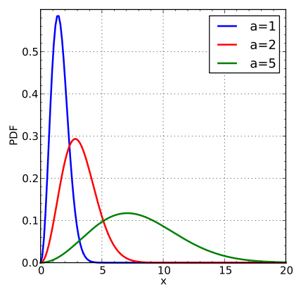
In statistics (and in probability theory), they call this a chi distribution with three degrees of freedom and a scale parameter which is equal to a = (kT/m)^1/2. The formula for the scale parameter shows how the mass of a particle indeed acts as a reverse scale parameter. The graph above shows three graphs for a = 1, 2 and 5 respectively. Note the square root though: quadrupling the mass (keeping kT the same) amounts to going from a = 2 to a = 1, so that’s halving a. Indeed, [kT/(4m)]^1/2 = (1/2)(kT/m)^1/2. So we can’t just do what we want with Δv (like multiplying it with 1836, as suggested). In fact, the graph and the formulas show that Feynman’s assumption that we can equate p with Δp (i.e. his assumption that “the momenta must be of the order p = ħ/Δx, with Δx the spread in position”), more or less at least, is quite reasonable.

Of course, you are very smart and so you’ll have yet another objection: why can’t we associate a much higher momentum with the proton, as that would allow us to associate higher velocities with the proton? Good question. My answer to that is the following (and it might be original, as I didn’t find this anywhere else). When everything is said and done, we’re talking two particles in some box here: an electron and a proton. Hence, we should assume that the average kinetic energy of our electron and our proton is the same (if not, they would be exchanging kinetic energy until it’s more or less equal), so we write <m_electron·v²_electron/2> = <m_proton·v²_proton/2>. We can re-write this as m_p/m_e = 1/1836 = <v²_e>/<v²_p> and, therefore, <v²_e> = 1836·<v²_p>. Now, <v²> ≠ <v>² and, hence, <v> ≠ √<v²>. So the equality does not imply that the expected velocity of the electron is √1836 ≈ 43 times the expected velocity of the proton. Indeed, because of the particularities of the distribution, there is a difference between (a) the most probable speed, which is equal to √2·a ≈ 1.414·a, (b) the root mean square speed, which is equal to √<v²> = √3·a ≈ 1.732·a, and, finally, (c) the mean or expected speed, which is equal to <v> = 2·(2/π)^1/2·a ≈ 1.596·a.

However, we are not far off. We could use any of these three values to roughly approximate Δv, as well as the scale parameter a itself: our answers would all be of the same order. However, to keep the calculations simple, let’s use the most probable speed. Let’s equate our electron mass with unity, so the mass of our proton is 1836. Now, such mass implies a scale factor (i.e. a) that’s √1836 ≈ 43 times smaller. So the most probable speed of the proton and, therefore, its spread, would be about √2/√1836 = √(2/1836) ≈ 0.033 that of the electron, so we write: Δv_p ≈ 0.033·Δv_e. Now we can insert this in our ΔxΔv = ħ/m = ħ/1836 identity. We get: Δx_pΔv_p = Δx_p·√(2/1836)·Δv_e = ħ/1836. That, in turn, implies that √(2·1836)·Δx_p = ħ/Δv_e, which we can re-write as: Δx_p = Δx_e/√(2·1836) ≈ Δx_e/60. In other words, the expected spread in the position of the proton is about 60 times smaller than the expected spread of the electron. More in general, we can say that the spread in position of a particle, keeping all else equal, is inversely proportional to (2m)^1/2. Indeed, in this case, we multiplied the mass with about 1800, and we found that the uncertainty in position went down with a factor 1/60 = 1/√3600. Not bad as a result ! Is it precise? Well… It could be like √3·√m or 2·(2/π)^1/2··√m depending on our definition of ‘uncertainty’, but it’s all of the same order. So… Yes. Not bad at all… 🙂

You’ll raise a third objection now: the radius of a proton is measured using the femtometer scale, so that’s expressed in 10⁻¹⁵ m, which is not 60 but a million times smaller than the nanometer (i.e. 10⁻⁹ m) scale used to express the Bohr radius as calculated by Feynman above. You’re right, but the 10⁻¹⁵ m number is the charge radius, not the uncertainty in position. Indeed, the so-called classical electron radius is also measured in femtometer and, hence, the Bohr radius is also like a million times that number. OK. That should settle the matter. I need to move on.

Before I do move on, let me relate the observation (i.e. the fact that the uncertainty in regard to position decreases as the mass of a particle increases) to another phenomenon. As you know, the interference of light beams is easy to observe. Hence, the interference of photons is easy to observe: Young’s experiment involved a slit of 0.85 mm (so almost 1 mm) only. In contrast, the 2012 double-slit experiment with electrons involved slits that were 62 nanometer wide, i.e. 62 billionths of a meter! That’s because the associated frequencies are so much higher and, hence, the wave zone is much smaller. So much, in fact, that Feynman could not imagine technology would ever be sufficiently advanced so as to actually carry out the double slit experiment with electrons. It’s an aspect of the same: the uncertainty in position is much smaller for electrons than it is for photons. Who knows: perhaps one day, we’ll be able to do the experiment with protons. 🙂 For further detail, I’ll refer you one of my posts on this.

What’s Explained, and What’s Left Unexplained?

There is another obvious question: if the electron is still some point charge, and going around as it does, why doesn’t it radiate energy? Indeed, the Rutherford-Bohr model had to be discarded because this ‘planetary’ model involved circular (or elliptical) motion and, therefore, some acceleration. According to classical theory, the electron should thus emit electromagnetic radiation, as a result of which it would radiate its kinetic energy away and, therefore, spiral in toward the nucleus. The quantum-mechanical model doesn’t explain this either, does it?

I can’t answer this question as yet, as I still need to go through all Feynman’s Lectures on quantum mechanics. You’re right. There’s something odd about the quantum-mechanical idea: it still involves a electron moving in some kind of orbital − although I hasten to add that the wavefunction is a complex-valued function, not some real function − but it does not involve any loss of kinetic energy due to circular motion apparently!

There are other unexplained questions as well. For example, the idea of an electrical point charge still needs to be re-conciliated with the mathematical inconsistencies it implies, as Feynman points out himself in yet another of his Lectures.

Finally, you’ll wonder as to the difference between a proton and a positron: if a positron and an electron annihilate each other in a flash, why do we have a hydrogen atom at all? Well… The proton is not the electron’s anti-particle. For starters, it’s made of quarks, while the positron is made of… Well… A positron is a positron: it’s elementary. But, yes, interesting question, and the ‘mechanics’ behind the mutual destruction are quite interesting and, hence, surely worth looking into—but not here. 🙂

Having mentioned a few things that remain unexplained, the model does have the advantage of solving plenty of other questions. It explains, for example, why the electron and the proton are actually right on top of each other, as they should be according to classical electrostatic theory, and why they are not at the same time: the electron is still a sort of ‘cloud’ indeed, with the proton at its center.

The quantum-mechanical ‘cloud’ model of the electron also explains why “the terrific electrical forces balance themselves out, almost perfectly, by forming tight, fine mixtures of the positive and the negative, so there is almost no attraction or repulsion at all between two separate bunches of such mixtures” (Richard Feynman, Introduction to Electromagnetism, p. 1-1) or, to quote from one of his other writings, why we do not fall through the floor as we walk:

“As we walk, our shoes with their masses of atoms push against the floor with its mass of atoms. In order to squash the atoms closer together, the electrons would be confined to a smaller space and, by the uncertainty principle, their momenta would have to be higher on the average, and that means high energy; the resistance to atomic compression is a quantum-mechanical effect and not a classical effect. Classically, we would expect that if we were to draw all the electrons and protons closer together, the energy would be reduced still further, and the best arrangement of positive and negative charges in classical physics is all on top of each other. This was well known in classical physics and was a puzzle because of the existence of the atom. Of course, the early scientists invented some ways out of the trouble—but never mind, we have the right way out, now!”

So that’s it, then. Except… Well…

The Fine-Structure Constant

When talking about the stability of atoms, one cannot escape a short discussion of the so-called fine-structure constant, denoted by α (alpha). I discussed it another post of mine, so I’ll refer you there for a more comprehensive overview. I’ll just remind you of the basics:

(1) α is the square of the electron charge expressed in Planck units: α = e_P².

(2) α is the square root of the ratio of (a) the classical electron radius and (b) the Bohr radius: α = √(r_e /r). You’ll see this more often written as r_e = α²r. Also note that this is an equation that does not depend on the units, in contrast to equation 1 (above), and 4 and 5 (below), which require you to switch to Planck units. It’s the square of a ratio and, hence, the units don’t matter. They fall away.

(3) α is the (relative) speed of an electron: α = v/c. [The relative speed is the speed as measured against the speed of light. Note that the ‘natural’ unit of speed in the Planck system of units is equal to c. Indeed, if you divide one Planck length by one Planck time unit, you get (1.616×10⁻³⁵ m)/(5.391×10⁻⁴⁴ s) = c m/s. However, this is another equation, just like (2), that does not depend on the units: we can express v and c in whatever unit we want, as long we’re consistent and express both in the same units.]

(4) Finally, α is also equal to the product of (a) the electron mass (which I’ll simply write as m_e here) and (b) the classical electron radius r_e (if both are expressed in Planck units): α = m_e·r_e. [I think that’s, perhaps, the most amazing of all of the expressions for α. If you don’t think that’s amazing, I’d really suggest you stop trying to study physics.]

Note that, from (2) and (4), we also find that:

(5) The electron mass (in Planck units) is equal m_e = α/r_e = α/α²r = 1/αr. So that gives us an expression, using α once again, for the electron mass as a function of the Bohr radius r expressed in Planck units.

Finally, we can also substitute (1) in (5) to get:

(6) The electron mass (in Planck units) is equal to m_e = α/r_e  = e_P²/r_e. Using the Bohr radius, we get m_e = 1/αr = 1/e_P²r.

In addition, in the mentioned post, I also related α to the so-called coupling constant determining the strength of the interaction between electrons and photons. So… What a magical number indeed ! It suggests some unity that our little model of the atom above doesn’t quite capture. As far as I am concerned, it’s one of the many other ‘unexplained questions’, and one of my key objectives, as I struggle through Feynman’s Lectures, is to understand it all. 🙂 One of the issues is, of course, how to relate this coupling constant to the concept of a gauge, which I briefly discussed in my previous post. In short, I’ve still got a long way to go… 😦

Post Scriptum: The de Broglie relations and the Uncertainty Principle

My little exposé on mass being nothing but a scale factor in the Uncertainty Principle is a good occasion to reflect on the Uncertainty Principle once more. Indeed, what’s the uncertainty about, if it’s not about the mass? It’s about the position in space and velocity, i.e. it’s movement and time. Velocity or speed (i.e. the magnitude of the velocity vector) is, in turn, defined as the distance traveled divided by the time of travel, so the uncertainty is about time as well, as evidenced from the ΔEΔt = h expression of the Uncertainty Principle. But how does it work exactly?

Hmm… Not sure. Let me try to remember the context. We know that the de Broglie relation, λ = h/p, which associates a wavelength (λ) with the momentum (p) of a particle, is somewhat misleading, because we’re actually associating a (possibly infinite) bunch of component waves with a particle. So we’re talking some range of wavelengths (Δλ) and, hence, assuming all these component waves travel at the same speed, we’re also talking a frequency range (Δf). The bottom line is that we’ve got a wave packet and we need to distinguish the velocity of its phase (v_p) versus the group velocity (v_g), which corresponds to the classical velocity of our particle.

I think I explained that pretty well in one of my previous posts on the Uncertainty Principle, so I’d suggest you have a look there. The mentioned post explains how the Uncertainty Principle relates position (x) and momentum (p) as a Fourier pair, and it also explains that general mathematical property of Fourier pairs: the more ‘concentrated’ one distribution is, the more ‘spread out’ its Fourier transform will be. In other words, it is not possible to arbitrarily ‘concentrate’ both distributions, i.e. both the distribution of x (which I denoted as Ψ(x) as well as its Fourier transform, i.e. the distribution of p (which I denoted by Φ(p)). So, if we’d ‘squeeze’ Ψ(x), then its Fourier transform Φ(p) will ‘stretch out’.

That was clear enough—I hope! But how do we go from ΔxΔp = h to ΔEΔt = h? Why are energy and time another Fourier pair? To answer that question, we need to clearly define what energy and what time we are talking about. The argument revolves around the second de Broglie relation: E = h·f. How do we go from the momentum p to the energy E? And how do we go from the wavelength λ to the frequency f?

The answer to the first question is the energy-mass equivalence: E = mc², always. This formula is relativistic, as m is the relativistic mass, so it includes the rest mass m₀ as well as the equivalent mass of its kinetic energy m₀v²/2 + … [Note, indeed, that the kinetic energy – defined as the excess energy over its rest energy – is a rapidly converging series of terms, so only the m₀v²/2 term is mentioned.] Likewise, momentum is defined as p = mv, always, with m the relativistic mass, i.e. m = (1−v²/c²)^−1/2·m₀ = γ·m₀, with γ the Lorentz factor. The E = mc² and p = mv relations combined give us the E/c = m·c = p·c/v or E·v/c = p·c relationship, which we can also write as E/p = c²/v. However, we’ll need to write E as a function of p for the purpose of a derivation. You can verify that E² − p²c² = m₀²c⁴) and, hence, that E = (p²c² + m₀²c⁴)^1/2.

Now, to go from a wavelength to a frequency, we need the wave velocity, and we’re obviously talking the phase velocity here, so we write: v_p = λ·f. That’s where the de Broglie hypothesis comes in: de Broglie just assumed the Planck-Einstein relation E = h·ν, in which ν is the frequency of a massless photon, would also be valid for massive particles, so he wrote: E = h·f. It’s just a hypothesis, of course, but it makes everything come out alright. More in particular, the phase velocity v_p = λ·f can now be re-written, using both de Broglie relations (i.e. h/p = λ and E/h = f) as v_p = (E/h)·(p/h) = E/p = c²/v. Now, because v is always smaller than c for massive particles (and usually very much smaller), we’re talking a superluminal phase velocity here! However, because it doesn’t carry any signal, it’s not inconsistent with relativity theory.

Now what about the group velocity? To calculate the group velocity, we need the frequencies and wavelengths of the component waves. The dispersion relation assumes the frequency of each component wave can be expressed as a function of its wavelength, so f = f(λ). Now, it takes a bit of wave mechanics (which I won’t elaborate on here) to show that the group velocity is the derivative of f with respect to λ, so we write v_g = ∂f/∂λ. Using the two de Broglie relations, we get: v_g = ∂f/∂λ = ∂(E/h)/∂(p/h) = ∂E/∂p = ∂[p²c² + m₀²c⁴)^1/2]/∂p. Now, when you write it all out, you should find that v_g = ∂f/∂λ = pc²/E = c²/v_p = v, so that’s the classical velocity of our particle once again.

Phew! Complicated! Yes. But so we still don’t have our ΔEΔt = h expression! All of the above tells us how we can associate a range of momenta (Δp) with a range of wavelengths (Δλ) and, in turn, with a frequency range (Δf) which then gives us some energy range (ΔE), so the logic is like:

Δp ⇒ Δλ ⇒ Δf ⇒ ΔE

Somehow, the same sequence must also ‘transform’ our Δx into Δt. I googled a bit, but I couldn’t find any clear explanation. Feynman doesn’t seem to have one in his Lectures either so, frankly, I gave up. What I did do in one of my previous posts, is to give some interpretation. However, I am not quite sure if it’s really the interpretation: there are probably several ones. It must have something to do with the period of a wave, but I’ll let you break your head over it. 🙂 As far as I am concerned, it’s just one of the other unexplained questions I have as I sort of close my study of ‘classical’ physics. So I’ll just make a mental note of it. [Of course, please don’t hesitate to send me your answer, if you’d have one!] Now it’s time to really dig into quantum mechanics, so I should really stay silent for quite a while now! 🙂

Some content on this page was disabled on June 16, 2020 as a result of a DMCA takedown notice from The California Institute of Technology. You can learn more about the DMCA here:

https://en.support.wordpress.com/copyright-and-the-dmca/