
Pre-script (dated 26 June 2020): This post has become less relevant (even irrelevant, perhaps) because my views on all things quantum-mechanical have evolved significantly as a result of my progression towards a more complete realist (classical) interpretation of quantum physics. I keep blog posts like these mainly because I want to keep track of where I came from. I might review them one day, but I currently don’t have the time or energy for it. 🙂
Original post:
I’ve written a few posts on the Uncertainty Principle already. See, for example, my post on the energy-time expression for it (ΔE·Δt ≥ h). So why am I coming back to it once more? Not sure. I felt I left some stuff out. So I am writing this post to just complement what I wrote before. I’ll do so by explaining, and commenting on, the ‘semi-formal’ derivation of the so-called Kennard formulation of the Principle in the Wikipedia article on it.
The Kennard inequalities, σxσp ≥ ħ/2 and σEσt ≥ ħ/2, are more accurate than the more general Δx·Δp ≥ h and ΔE·Δt ≥ h expressions one often sees, which are an early formulation of the Principle by Niels Bohr, and which Heisenberg himself used when explaining the Principle in a thought experiment picturing a gamma-ray microscope. I presented Heisenberg’s thought experiment in another post, and so I won’t repeat myself here. I just want to mention that it ‘proves’ the Uncertainty Principle using the Planck-Einstein relations for the energy and momentum of a photon:
E = hf and p = h/λ
Heisenberg’s thought experiment is not a real proof, of course. But then what’s a real proof? The mentioned ‘semi-formal’ derivation looks more impressive, because more mathematical, but it’s not a ‘proof’ either (I hope you’ll understand why I am saying that after reading my post). The main difference between Heisenberg’s thought experiment and the mathematical derivation in the mentioned Wikipedia article is that the ‘mathematical’ approach is based on the de Broglie relation. That de Broglie relation looks the same as the Planck-Einstein relation (p = h/λ) but it’s fundamentally different.
Indeed, the momentum of a photon (i.e. the p we use in the Planck-Einstein relation) is not the momentum one associates with a proper particle, such as an electron or a proton, for example (so that’s the p we use in the de Broglie relation). The momentum of a particle is defined as the product of its mass (m) and velocity (v). Photons don’t have a (rest) mass, and their velocity is absolute (c), so how do we define momentum for a photon? There are a couple of ways to go about it, but the two most obvious ones are probably the following:
- We can use the classical theory of electromagnetic radiation and show that the momentum of a photon is related to the magnetic field (we usually only analyze the electric field), and the so-called radiation pressure that results from it. It yields the p = E/c formula which we need to go from E = hf to p = h/λ, using the ubiquitous relation between the frequency, the wavelength and the wave velocity (c = λf). In case you’re interested in the detail, just click on the radiation pressure link).
- We can also use the mass-energy equivalence E = mc2. Hence, the equivalent mass of the photon is E/c2, which is relativistic mass only. However, we can multiply that mass with the photon’s velocity, which is c, thereby getting the very same value for its momentum p = c·E/c2 = E/c.
So Heisenberg’s ‘proof’ uses the Planck-Einstein relations, as it analyzes the Uncertainty Principle more as an observer effect: probing matter with light, so to say. In contrast, the mentioned derivation takes the de Broglie relation itself as the point of departure. As mentioned, the de Broglie relations look exactly the same as the Planck-Einstein relationship (E = hf and p = h/λ) but the model behind is very different. In fact, that’s what the Uncertainty Principle is all about: it says that the de Broglie frequency and/or wavelength cannot be determined exactly: if we want to localize a particle, somewhat at least, we’ll be dealing with a frequency range Δf. As such, the de Broglie relation is actually somewhat misleading at first. Let’s talk about the model behind.
A particle, like an electron or a proton, traveling through space, is described by a complex-valued wavefunction, usually denoted by the Greek letter psi (Ψ) or phi (Φ). This wavefunction has a phase, usually denoted as θ (theta) which – because we assume the wavefunction is a nice periodic function – varies as a function of time and space. To be precise, we write θ as θ = ωt – kx or, if the wave is traveling in the other direction, as θ = kx – ωt.
I’ve explained this in a couple of posts already, including my previous post, so I won’t repeat myself here. Let me just note that ω is the angular frequency, which we express in radians per second, rather than cycles per second, so ω = 2πf (one cycle covers 2π rad). As for k, that’s the wavenumber, which is often described as the spatial frequency, because it’s expressed in cycles per meter or, more often (and surely in this case), in radians per meter. Hence, if we freeze time, this number is the rate of change of the phase in space. Because one cycle is, again, 2π rad, and one cycle corresponds to the wave traveling one wavelength (i.e. λ meter), it’s easy to see that k = 2π/λ. We can use these definitions to re-write the de Broglie relations E = hf and p = h/λ as:
E = ħω and p = ħk with h = h/2π
What about the wave velocity? For a photon, we have c = λf and, hence, c = (2π/k)(ω/2π) = ω/k. For ‘particle waves’ (or matter waves, if you prefer that term), it’s much more complicated, because we need to distinguish between the so-called phase velocity (vp) and the group velocity (vg). The phase velocity is what we’re used to: it’s the product of the frequency (the number of cycles per second) and the wavelength (the distance traveled by the wave over one cycle), or the ratio of the angular frequency and the wavenumber, so we have, once again, λf = ω/k = vp. However, this phase velocity is not the classical velocity of the particle that we are looking at. That’s the so-called group velocity, which corresponds to the velocity of the wave packet representing the particle (or ‘wavicle’, if your prefer that term), as illustrated below.

The animation below illustrates the difference between the phase and the group velocity even more clearly: the green dot travels with the ‘wavicles’, while the red dot travels with the phase. As mentioned above, the group velocity corresponds to the classical velocity of the particle (v). However, the phase velocity is a mathematical point that actually travels faster than light. It is a mathematical point only, which does not carry a signal (unlike the modulation of the wave itself, i.e. the traveling ‘groups’) and, hence, it does not contradict the fundamental principle of relativity theory: the speed of light is absolute, and nothing travels faster than light (except mathematical points, as you can, hopefully, appreciate now).

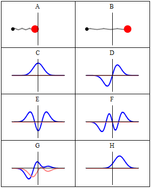
The two animations above do not represent the quantum-mechanical wavefunction, because the functions that are shown are real-valued, not complex-valued. To imagine a complex-valued wave, you should think of something like the ‘wavicle’ below or, if you prefer animations, the standing waves underneath (i.e. C to H: A and B just present the mathematical model behind, which is that of a mechanical oscillator, like a mass on a spring indeed). These representations clearly show the real as well as the imaginary part of complex-valued wave-functions.

With this general introduction, we are now ready for the more formal treatment that follows. So our wavefunction Ψ is a complex-valued function in space and time. A very general shape for it is one we used in a couple of posts already:
Ψ(x, t) ∝ ei(kx – ωt) = cos(kx – ωt) + isin(kx – ωt)
If you don’t know anything about complex numbers, I’d suggest you read my short crash course on it in the essentials page of this blog, because I don’t have the space nor the time to repeat all of that. Now, we can use the de Broglie relationship relating the momentum of a particle with a wavenumber (p = ħk) to re-write our psi function as:
Ψ(x, t) ∝ ei(kx – ωt) = ei(px/ħ – ωt)
Note that I am using the ‘proportional to’ symbol (∝) because I don’t worry about normalization right now. Indeed, from all of my other posts on this topic, you know that we have to take the absolute square of all these probability amplitudes to arrive at a probability density function, describing the probability of the particle effectively being at point x in space at point t in time, and that all those probabilities, over the function’s domain, have to add up to 1. So we should insert some normalization factor.
Having said that, the problem with the wavefunction above is not normalization really, but the fact that it yields a uniform probability density function. In other words, the particle position is extremely uncertain in the sense that it could be anywhere. Let’s calculate it using a little trick: the absolute square of a complex number equals the product of itself with its (complex) conjugate. Hence, if z = reiθ, then │z│2 = zz* = reiθ·re–iθ = r2eiθ–iθ = r2e0 = r2. Now, in this case, assuming unique values for k, ω, p, which we’ll note as k0, ω0, p0 (and, because we’re freezing time, we can also write t = t0), we should write:
│Ψ(x)│2 = │a0ei(p0x/ħ – ω0t0) │2 = │a0eip0x/ħ e–iω0t0 │2 = │a0eip0x/ħ │2 │e–iω0t0 │2 = a02
Note that, this time around, I did insert some normalization constant a0 as well, so that’s OK. But so the problem is that this very general shape of the wavefunction gives us a constant as the probability for the particle being somewhere between some point a and another point b in space. More formally, we get the surface for a rectangle when we calculate the probability P[a ≤ X ≤ b] as we should calculate it, which is as follows:

More specifically, because we’re talking one-dimensional space here, we get P[a ≤ X ≤ b] = (b–a)·a02. Now, you may think that such uniform probability makes sense. For example, an electron may be in some orbital around a nucleus, and so you may think that all ‘points’ on the orbital (or within the ‘sphere’, or whatever volume it is) may be equally likely. Or, in another example, we may know an electron is going through some slit and, hence, we may think that all points in that slit should be equally likely positions. However, we know that it is not the case. Measurements show that not all points are equally likely. For an orbital, we get complicated patterns, such as the one shown below, and please note that the different colors represent different complex numbers and, hence, different probabilities.

Also, we know that electrons going through a slit will produce an interference pattern—even if they go through it one by one! Hence, we cannot associate some flat line with them: it has to be a proper wavefunction which implies, once again, that we can’t accept a uniform distribution.
In short, uniform probability density functions are not what we see in Nature. They’re non-uniform, like the (very simple) non-uniform distributions shown below. [The left-hand side shows the wavefunction, while the right-hand side shows the associated probability density function: the first two are static (i.e. they do not vary in time), while the third one shows a probability distribution that does vary with time.]

I should also note that, even if you would dare to think that a uniform distribution might be acceptable in some cases (which, let me emphasize this, it is not), an electron can surely not be ‘anywhere’. Indeed, the normalization condition implies that, if we’d have a uniform distribution and if we’d consider all of space, i.e. if we let a go to –∞ and b to +∞, then a02 would tend to zero, which means we’d have a particle that is, literally, everywhere and nowhere at the same time.
In short, a uniform probability distribution does not make sense: we’ll generally have some idea of where the particle is most likely to be, within some range at least. I hope I made myself clear here.
Now, before I continue, I should make some other point as well. You know that the Planck constant (h or ħ) is unimaginably small: about 1×10⁻³⁴ J·s (joule-second). In fact, I’ve repeatedly made that point in various posts. However, having said that, I should add that, while it’s unimaginably small, the uncertainties involved are quite significant. Let us indeed look at the value of ħ by relating it to that σxσp ≥ ħ/2 relation.
Let’s first look at the units. The uncertainty in the position should obviously be expressed in distance units, while momentum is expressed in kg·m/s units. So that works out, because 1 joule is the energy transferred (or work done) when applying a force of 1 newton (N) over a distance of 1 meter (m). In turn, one newton is the force needed to accelerate a mass of one kg at the rate of 1 meter per second per second (this is not a typing mistake: it’s an acceleration of 1 m/s per second, so the unit is m/s2: meter per second squared). Hence, 1 J·s = 1 N·m·s = 1 kg·m/s2·m·s = kg·m2/s. Now, that’s the same dimension as the ‘dimensional product’ for momentum and distance: m·kg·m/s = kg·m2/s.
Now, these units (kg, m and s) are all rather astronomical at the atomic scale and, hence, h and ħ are usually expressed in other dimensions, notably eV·s (electronvolt-second). However, using the standard SI units gives us a better idea of what we’re talking about. If we split the ħ = 1×10⁻³⁴ J·s value (let’s forget about the 1/2 factor for now) ‘evenly’ over σx and σp – whatever that means: all depends on the units, of course! – then both factors will have magnitudes of the order of 1×10⁻¹⁷: 1×10−17 m times 1×10−17 kg·m/s gives us 1×10⁻³⁴ J·s.
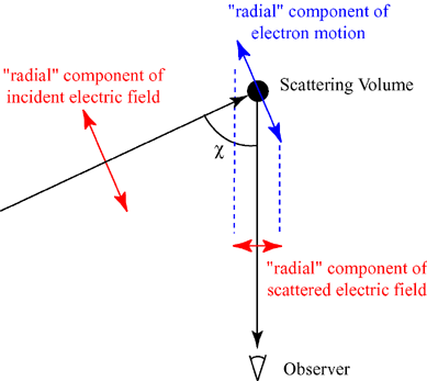
You may wonder how this 1×10⁻¹⁷ m compares to, let’s say, the classical electron radius, for example. The classical electron radius is, roughly speaking, the ‘space’ an electron seems to occupy as it scatters incoming light. The idea is illustrated below (credit for the image goes to Wikipedia, as usual). The classical electron radius – or Thompson scattering length – is about 2.818×10⁻¹⁵ m, so that’s almost 300 times our ‘uncertainty’ (1×10⁻¹⁷ m). Not bad: it means that we can effectively relate our ‘uncertainty’ in regard to the position to some actual dimension in space. In this case, we’re talking the femtometer scale (1 fm = 10−15 m), and so you’ve surely heard of this before.
What about the other ‘uncertainty’, the one for the momentum (1×10⁻¹⁷ kg·m/s)? What’s the typical (linear) momentum of an electron? Its mass, expressed in kg, is about 9.1×10⁻³¹ kg. We also know its relative velocity in an electron: it’s that magical number α = v/c, about which I wrote in some other posts already, so v = αc ≈ 0.0073·3×108 m/s ≈ 2.2×10⁶ m/s. Now, 9.1×10−31 kg times 2.2×106 m/s is about 2×10–26 kg·m/s, so our proposed ‘uncertainty’ in regard to the momentum (1×10⁻¹⁷ kg·m/s) is half a billion times larger than the typical value for it. Now that is, obviously, not so good. [Note that calculations like this are extremely rough. In fact, when one talks electron momentum, it’s usual angular momentum, which is ‘analogous’ to linear momentum, but angular momentum involves very different formulas. If you want to know more about this, check my post on it.]
Of course, now you may feel that we didn’t ‘split’ the uncertainty in a way that makes sense: those –17 exponents don’t work, obviously. So let’s take 1×10–26 kg·m/s for σp, which is half of that ‘typical’ value we calculated. Then we’d have 1×10⁻⁸ m for σx (1×10−8 m times 1×10–26 kg·m/s is, once again, 1×10–34 J·s). But then that uncertainty suddenly becomes a huge number: 1×10⁻⁸ m is 100 angstrom. That’s not the atomic scale but the molecular scale! So it’s huge as compared to the pico- or femto-meter scale (1 pm = 1×10⁻¹² m, 1 fm = 1×10⁻¹⁵ m) which we’d sort of expect to see when we’re talking electrons.
OK. Let me get back to the lesson. Why this digression? Not sure. I think I just wanted to show that the Uncertainty Principle involves ‘uncertainties’ that are extremely relevant: despite the unimaginable smallness of the Planck constant, these uncertainties are quite significant at the atomic scale. But back to the ‘proof’ of Kennard’s formulation. Here we need to discuss the ‘model’ we’re using. The rather simple animation below (again, credit for it has to go to Wikipedia) illustrates it wonderfully.

Look at it carefully: we start with a ‘wave packet’ that looks a bit like a normal distribution, but it isn’t, of course. We have negative and positive values, and normal distributions don’t have that. So it’s a wave alright. Of course, you should, once more, remember that we’re only seeing one part of the complex-valued wave here (the real or imaginary part—it could be either). But so then we’re superimposing waves on it. Note the increasing frequency of these waves, and also note how the wave packet becomes increasingly localized with the addition of these waves. In fact, the so-called Fourier analysis, of which you’ve surely heard before, is a mathematical operation that does the reverse: it separates a wave packet into its individual component waves.
So now we know the ‘trick’ for reducing the uncertainty in regard to the position: we just add waves with different frequencies. Of course, different frequencies imply different wavenumbers and, through the de Broglie relationship, we’ll also have different values for the ‘momentum’ associated with these component waves. Let’s write these various values as kn, ωn, and pn respectively, with n going from 0 to N. Of course, our point in time remains frozen at t0. So we get a wavefunction that’s, quite simply, the sum of N component waves and so we write:
Ψ(x) = ∑ anei(pnx/ħ – ωnt0) = ∑ an eipnx/ħe–iωnt0 = ∑ Aneipnx/ħ
Note that, because of the e–iωnt0, we now have complex-valued coefficients An = ane–iωnt0 in front. More formally, we say that An represents the relative contribution of the mode pn to the overall Ψ(x) wave. Hence, we can write these coefficients A as a function of p. Because Greek letters always make more of an impression, we’ll use the Greek letter Φ (phi) for it. 🙂 Now, we can go to the continuum limit and, hence, transform that sum above into an infinite sum, i.e. an integral. So our wave function then becomes an integral over all possible modes, which we write as:

Don’t worry about that new 1/√2πħ factor in front. That’s, once again, something that has to do with normalization and scales. It’s the integral itself you need to understand. We’ve got that Φ(p) function there, which is nothing but our An coefficient, but for the continuum case. In fact, these relative contributions Φ(p) are now referred to as the amplitude of all modes p, and so Φ(p) is actually another wave function: it’s the wave function in the so-called momentum space.
You’ll probably be very confused now, and wonder where I want to go with an integral like this. The point to note is simple: if we have that Φ(p) function, we can calculate (or derive, if you prefer that word) the Ψ(x) from it using that integral above. Indeed, the integral above is referred to as the Fourier transform, and it’s obviously closely related to that Fourier analysis we introduced above.
Of course, there is also an inverse transform, which looks exactly the same: it just switches the wave functions (Ψ and Φ) and variables (x and p), and then (it’s an important detail!), it has a minus sign in the exponent. Together, the two functions – as defined by each other through these two integrals – form a so-called Fourier integral pair, also known as a Fourier transform pair, and the variables involved are referred to as conjugate variables. So momentum (p) and position (x) are conjugate variables and, likewise, energy and time are also conjugate variables (but so I won’t expand on the time-energy relation here: please have a look at one of my others posts on that).
Now, I thought of copying and explaining the proof of Kennard’s inequality from Wikipedia’s article on the Uncertainty Principle (you need to click on the show button in the relevant section to see it), but then that’s pretty boring math, and simply copying stuff is not my objective with this blog. More importantly, the proof has nothing to do with physics. Nothing at all. Indeed, it just proves a general mathematical property of Fourier pairs. More specifically, it proves that, the more concentrated one function is, the more spread out its Fourier transform must be. In other words, it is not possible to arbitrarily concentrate both a function and its Fourier transform.
So, in this case, if we’d ‘squeeze’ Ψ(x), then its Fourier transform Φ(p) will ‘stretch out’, and so that’s what the proof in that Wikipedia article basically shows. In other words, there is some ‘trade-off’ between the ‘compaction’ of Ψ(x), on the one hand, and Φ(p), on the other, and so that is what the Uncertainty Principle is all about. Nothing more, nothing less.
But… Yes? What’s all this talk about ‘squeezing’ and ‘compaction’? We can’t change reality, can we? Well… Here we’re entering the philosophical field, of course. How do we interpret the Uncertainty Principle? It surely does look like us trying to measure something has some impact on the wavefunction. In fact, usually, our measurement – of either position or momentum – usually makes the wavefunctions collapse: we suddenly know where the particle is and, hence, ψ(x) seems to collapse into one point. Alternatively, we measure its momentum and, hence, Φ(p) collapses.
That’s intriguing. In fact, even more intriguing is the possibility we may only partially affect those wavefunctions with measurements that are somewhat less ‘drastic’. It seems a lot of research is focused on that (just Google for partial collapse of the wavefunction, and you’ll finds tons of references, including presentations like this one).
Hmm… I need to further study the topic. The decomposition of a wave into its component waves is obviously something that works well in physics—and not only in quantum mechanics but also in much more mundane examples. Its most general application is signal processing, in which we decompose a signal (which is a function of time) into the frequencies that make it up. Hence, our wavefunction model makes a lot of sense, as it mirrors the physics involved in oscillators and harmonics obviously.
Still… I feel it doesn’t answer the fundamental question: what is our electron really? What do those wave packets represent? Physicists will say questions like this don’t matter: as long as our mathematical models ‘work’, it’s fine. In fact, if even Feynman said that nobody – including himself – truly understands quantum mechanics, then I should just be happy and move on. However, for some reason, I can’t quite accept that. I should probably focus some more on that de Broglie relationship, p = h/λ, as it’s obviously as fundamental to my understanding of the ‘model’ of reality in physics as that Fourier analysis of the wave packet. So I need to do some more thinking on that.
The de Broglie relationship is not intuitive. In fact, I am not ashamed to admit that it actually took me quite some time to understand why we can’t just re-write the de Broglie relationship (λ = h/p) as an uncertainty relation itself: Δλ = h/Δp. Hence, let me be very clear on this:
Δx = h/Δp (that’s the Uncertainty Principle) but Δλ ≠ h/Δp !
Let me quickly explain why.
If the Δ symbol expresses a standard deviation (or some other measurement of uncertainty), we can write the following:
p = h/λ ⇒ Δp = Δ(h/λ) = hΔ(1/λ) ≠ h/Δp
So I can take h out of the brackets after the Δ symbol, because that’s one of the things that’s allowed when working with standard deviations. More in particular, one can prove the following:
- The standard deviation of some constant function is 0: Δ(k) = 0
- The standard deviation is invariant under changes of location: Δ(x + k) = Δ(x + k)
- Finally, the standard deviation scales directly with the scale of the variable: Δ(kx) = |k |Δ(x).
However, it is not the case that Δ(1/x) = 1/Δx. However, let’s not focus on what we cannot do with Δx: let’s see what we can do with it. Δx equals h/Δp according to the Uncertainty Principle—if we take it as an equality, rather than as an inequality, that is. And then we have the de Broglie relationship: p = h/λ. Hence, Δx must equal:
Δx = h/Δp = h/[Δ(h/λ)] =h/[hΔ(1/λ)] = 1/Δ(1/λ)
That’s obvious, but so what? As mentioned, we cannot write Δx = Δλ, because there’s no rule that says that Δ(1/λ) = 1/Δλ and, therefore, h/Δp ≠ Δλ. However, what we can do is define Δλ as an interval, or a length, defined by the difference between its lower and upper bound (let’s denote those two values by λa and λb respectively. Hence, we write Δλ = λb – λa. Note that this does not assume we have a continuous range of values for λ: we can have any number of frequencies λn between λa and λb, but so you see the point: we’ve got a range of values λ, discrete or continuous, defined by some lower and upper bound.
Now, the de Broglie relation associates two values pa and pb with λa and λb respectively: pa = h/λa and pb = h/λb. Hence, we can similarly define the corresponding Δp interval as pa – pb, with pa = h/λa and pb = h/λb. Note that, because we’re taking the reciprocal, we have to reverse the order of the values here: if λb > λa, then pa = h/λa > pb = h/λb. Hence, we can write Δp = Δ(h/λ) = pa – pb = h/λ1 – h/λ2 = h(1/λ1 – 1/λ2) = h[λ2 – λ1]/λ1λ2. In case you have a bit of difficulty, just draw some reciprocal functions (like the ones below), and have fun connecting intervals on the horizontal axis with intervals on the vertical axis using these functions.

Now, h[λ2 – λ1]/λ1λ2) is obviously something very different than h/Δλ = h/(λ2 – λ1). So we can surely not equate the two and, hence, we cannot write that Δp = h/Δλ.
Having said that, the Δx = 1/Δ(1/λ) = λ1λ2/(λ2 – λ1) that emerges here is quite interesting. We’ve got a ratio here, λ1λ2/(λ2 – λ1, which shows that Δx depends only on the upper and lower bounds of the Δλ range. It does not depend on whether or not the interval is discrete or continuous.
The second thing that is interesting to note is Δx depends not only on the difference between those two values (i.e. the length of the interval) but also on their value: if the length of the interval, i.e. the difference between the two frequencies is the same, but their values as such are higher, then we get a higher value for Δx, i.e. a greater uncertainty in the position. Again, this shows that the relation between Δλ and Δx is not straightforward. But so we knew that already, and so I’ll end this post right here and right now. 🙂
Some content on this page was disabled on June 17, 2020 as a result of a DMCA takedown notice from Michael A. Gottlieb, Rudolf Pfeiffer, and The California Institute of Technology. You can learn more about the DMCA here:

One thought on “The Uncertainty Principle revisited”