
Pre-script (dated 26 June 2020): This post got mutilated by the removal of some illustrations by the dark force. You should be able to follow the main story-line, however. If anything, the lack of illustrations might actually help you to think things through for yourself.
Original post:
In my previous post, I mentioned the so-called method of images, but didn’t elaborate much. Let’s recall the problem. As you know, the whole subject of electrostatics is governed by one equation: the so-called Poisson equation:
∇2Φ = ∂2Φ/∂x2 + ∂2Φ/∂x2 + ∂2Φ/∂x2 = −ρ/ε0
We get this equation by combining Maxwell’s first law (∇·Φ = −ρ/ε0) and the E = −∇Φ formula. Now, if we know the distribution of charges, then we don’t need that Poisson equation: we can calculate the potential at every point – denoted by (1) below – using the following formulas:

And if we have Φ, we have E, because E = –∇Φ. But, in most actual situations, we don’t know the charge distribution, and then we need to work with that Poisson equation. Of course, you’ll say: if you don’t know the charge distribution, then you don’t know the ρ in the equation, and so what use is it really?
The answer is: most problems will involve conductors, and we do know that their surface is an equipotential surface. We also know that the electric field just outside the surface must be normal to the surface. Let’s take the example of the grounded conducting sheet once again, as depicted below. We know the image charge and the field lines on the left-hand side are not there. In fact, because the sheet is grounded, there is no net charge on it, and the conductor acts as a shield.

We do have a real field on the right-hand side though, and it’s exactly the same as that of a dipole: we only need to cross out the left-hand half of the picture. What charges are responsible for it? It surely cannot be the lone +q charge alone, and it’s isn’t: we also have induced local charges on the sheet. Indeed, the positive charge will attract negative charges to the surface and, hence, while the sheet as a whole is neutral (so it has no net charge), the surface charge density is not zero. We can calculate it. How? It’s quite complicated, but let’s give it a try.
Look at the detail below. Let’s forget about the induced charges for a while, and analyze the field produced by the positive charge in the absence of induced charges, so that’s the E field at point P. The magnitude of its normal component is En+ = E·cosθ, with θ the angle between the two vectors.
θ is an angle of a rectangular triangle, and it’s easy to see that cosθ is equal to a/(a2 + ρ2)1/2. Now, Coulomb’s Law tells us that E = (1/4πε0)·q/[(a2 + ρ2)1/2]2 = (1/4πε0)·q/(a2 + ρ2). Hence, we can write:
En+ = (1/4πε0)·a·q/(a2 + ρ2)3/2
[A quick note on the symbols used here: we use ρ (rho) to denote a distance here. That’s somewhat confusing because it usually denotes a volume density. However, we’re interested in a surface density here, for which the σ (sigma) symbol is used. So don’t worry about it. Just note that ρ is some distance here, instead of a charge density.]
Now we know that the induced charges will arrange themselves in such way that the addition of their field makes the field at P look like there was a negative charge of the same magnitude as q at the other side of the sheet. If there was such charge −q, then we could do the same analysis, as shown below. It’s easy to see that the component of the imaginary field along the sheet (i.e. the component that’s perpendicular to the normal) cancels the actual component along the shield of the field created by +q, while its normal component adds to the normal component of the +q field. To make a long story short, the actual field at P is equal to E(ρ) = (1/4πε0)·2a·q/(a2 + ρ2)3/2, and it has two components of strength (1/4πε0)·a·q/(a2 + ρ2)3/2.
To put it differently, the actual field can be thought as two parts: (1) the (normal) component of the field caused by + q, and (2) the field caused by the surface charge density σ at P, which we denote as σ(ρ). Let’s see what we can do with this.
The analysis of the field of a sheet of charge on a conductor is quite complicated, and not quite like the analysis of just a sheet of charge. The analysis for just a sheet of charge was based on the theoretical situation depicted below. We imagined some box with two Gaussian surfaces of area A, and we then used Gauss’ Law to deduce that, if σ was the charge per unit area (i.e. the surface density), the total flux out of the box should be equal to EA + EA = σA/ε0 and, hence, E = (1/2)·σ/ε0. The illustration below shows we should think of two fields with opposite direction, and with a magnitude of (1/2)·σ/ε0 each.
That’s simple enough. However, a sheet of charge on a conductor produces a different field, as shown below. Because of the shielding effect, we have flux on one side of the box only, and the field strength of this flux is σ/ε0, so that’s two times the (1/2)·σ/ε0 magnitude described above. However, as mentioned, it’s zero on the other side, i.e. the inside of the conductor shown below.
So what happens here? The charges in the neighborhood of a point P on the surface actually do produce a local field (Elocal), both inside and outside of the surface, which respects the Elocal = (1/2)·σ/2ε0 equality, but all the rest of the charges on the conductor “conspire” to produce an additional field at the point P, which also produces two fields, again with opposite direction and with a magnitude of (1/2)·σ/ε0 each. So the net result is that the total field inside goes to zero, and the field outside is equal to E = σ/ε0, so E = 2·Elocal. Note that the example above assumes a positively charged conductor: if the charge on the conductor would be negative, the direction of the field would be inwards, but we’d still have a field on and outside of the surface only.
I know you’ve switched off already but − just in case you didn’t − what equality should we use to find σ in this case, i.e. the grounded sheet with no net charge on it but with some (negative) surface charge density. Well… We’re talking a surface density, and a conductor, and, therefore, I would think it’s the E = σ/ε0, i.e. the formula for a charged sheet on a conductor. So we write:
E = σ(ρ)/ε0 ⇔ σ(ρ) = ε0E
But what E do we take to continue our calculation? The whole field or (1/4πε0)·a·q/(a2 + ρ2)3/2 only? The analysis above may make you think that we should take (1/4πε0)·a·q/(a2 + ρ2)3/2 only, so that’s the component that’s related to the imaginary charge only, but… No! We’re talking one actual field here, which is produced by the positive charge as well as by the induced charges. So we should not cut it for the purpose of calculating σ(ρ)! So the grand result is:
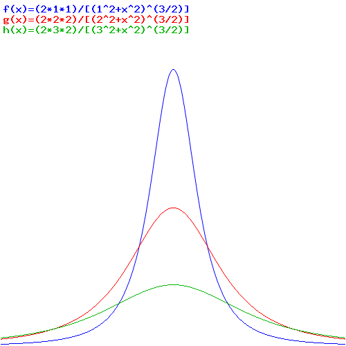
σ(ρ) = ε0E = (1/4π)·2a·q/(a2 + ρ2)3/2
The shape of this function should not surprise us: it’s shown below for some different values of q (1 and 2 respectively) and a (1, 2 and 3 respectively).
How do we know our solution is correct? We can check it: if we integrate σ over the whole surface, we should find that the total induced charge is equal to −q. So… Well… I’ll let you do that. Feynman also notes the induced charges should exert a force on our point charge, which we can calculating the force between the surface charges and the charge. It’s again an integral, and it should be equal to
![]()
Lo and behold! The force acting on the positive charge is exactly the same as it would be with the negative image charge instead of the plate. Why? Well… Because the fields are the same!
The results we obtained are quite wonderful! Indeed, we said we did not know the charge distribution, and so we used a very different method to find the field: the method of images, which consists of computing the field due to q and some imaginary point charge –q somewhere else. Feynman summarizes the method of images as follows:
“The point charge we “imagine” existing behind the conducting surface is called an image charge. In books you can find long lists of solutions for hyperbolic-shaped conductors and other complicated looking things, and you wonder how anyone ever solved these terrible shapes. They were solved backwards! Someone solved a simple problem with given charges. He then saw that some equipotential surface showed up in a new shape, and he wrote a paper in which he pointed out that the field outside that particular shape can be described in a certain way.”
However, as you can see, the method is actually quite powerful, because we got a substantial bonus here: we calculated the field indeed, but then we could also calculate the charge distribution afterwards, so we got it all! Let’s see if we master the topic by looking at some other applications of the method of images.
Point charges near conducting spheres
For a grounded conducting sphere, we get the result shown below: the point charge q will induce charges on it whose fields are those of an image charge q’ = −aq/b placed at the point below.
You can check the details in Feynman’s Lecture on it, in which you will also find a more general formula for spheres that are not at zero potential. The more general formula involves a third charge q” at the center of the sphere, with charge q” = −q’ = aq/b.
Again, we’ll have a force of attraction between the sphere and the point charge, even if the net charge on the sphere is zero, because it’s grounded. Indeed, the positive charge q attracts negative charges to the side closer to itself and, hence, leaves positive charges on the surface of the far side. As the attraction by the negative charges exceeds the repulsion from the positive charges, we end up with some net attraction. Feynman leaves us with an interesting challenge here:
“Those who were entertained in childhood by the baking powder box which has on its label a picture of a baking powder box which has on its label a picture of a baking powder box which has … may be interested in the following problem. Two equal spheres, one with a total charge of +Q and the other with a total charge of −Q, are placed at some distance from each other. What is the force between them? The problem can be solved with an infinite number of images. One first approximates each sphere by a charge at its center. These charges will have image charges in the other sphere. The image charges will have images, etc., etc., etc. The solution is like the picture on the box of baking powder—and it converges pretty fast.”
Well… I’ll leave it to you to take up that challenge. 🙂
Direct and indirect methods
Let me end this post by noting that I started out with that Poisson equation, but that I actually didn’t use it. Having said that, this method of images did result in some solutions for it. It is what Feynman calls an indirect method of solving some problems, and he writes the following on it:
“If the problem to be solved does not belong to the class of problems for which we can construct solutions by the indirect method, we are forced to solve the problem by a more direct method. The mathematical problem of the direct method is the solution of Laplace’s equation ∇2Φ = 0 subject to the condition that Φ is a suitable constant on certain boundaries—the surfaces of the conductors. [Note that Laplace’s equation is Poisson’s equation with a zero on the right-hand side.] Problems which involve the solution of a differential field equation subject to certain boundary conditions are called boundary-value problems. They have been the object of considerable mathematical study. In the case of conductors having complicated shapes, there are no general analytical methods. Even such a simple problem as that of a charged cylindrical metal can closed at both ends—a beer can—presents formidable mathematical difficulties. It can be solved only approximately, using numerical methods. The only general methods of solution are numerical.”
Well… That says it all, I guess. There are other indirect methods, i.e. other than the method of images, but I won’t present these here. I may write something about it in some other post, perhaps. 🙂
Some content on this page was disabled on June 16, 2020 as a result of a DMCA takedown notice from The California Institute of Technology. You can learn more about the DMCA here:
https://wordpress.com/support/copyright-and-the-dmca/
Some content on this page was disabled on June 16, 2020 as a result of a DMCA takedown notice from The California Institute of Technology. You can learn more about the DMCA here:https://wordpress.com/support/copyright-and-the-dmca/
Some content on this page was disabled on June 16, 2020 as a result of a DMCA takedown notice from The California Institute of Technology. You can learn more about the DMCA here:https://wordpress.com/support/copyright-and-the-dmca/
Some content on this page was disabled on June 16, 2020 as a result of a DMCA takedown notice from The California Institute of Technology. You can learn more about the DMCA here:https://wordpress.com/support/copyright-and-the-dmca/
Some content on this page was disabled on June 16, 2020 as a result of a DMCA takedown notice from The California Institute of Technology. You can learn more about the DMCA here:

Did anyone solve the two spheres problem?