Quantum-mechanical operators

I wrote a post on quantum-mechanical operators some while ago but, when re-reading it now, I am not very happy about it, because it tries to cover too much ground in one go. In essence, I regret my attempt to constantly switch between the matrix representation of quantum physics – with the | state 〉 symbols – and the wavefunction approach, so as to show how the operators work for both cases. But then that’s how Feynman approaches this.

However, let’s admit it: while Heisenberg’s matrix approach is equivalent to Schrödinger’s wavefunction approach – and while it’s the only approach that works well for n-state systems – the wavefunction approach is more intuitive, because:

1. Most practical examples of quantum-mechanical systems (like the description of the electron orbitals of an atomic system) involve continuous coordinate spaces, so we have an infinite number of states and, hence, we need to describe it using the wavefunction approach.
2. Most of us are much better-versed in using derivatives and integrals, as opposed to matrix operations.
3. A more intuitive statement of the same argument above is the following: the idea of one state flowing into another, rather than being transformed through some matrix, is much more appealing. 🙂

So let’s stick to the wavefunction approach here. So, while you need to remember that there’s a ‘matrix equivalent’ for each of the equations we’re going to use in this post, we’re not going to talk about it.

The operator idea

In classical physics – high school physics, really – we would describe a pointlike particle traveling in space by a function relating its position (x) to time (t): x = x(t). Its (instantaneous) velocity is, obviously, v(t) = dx/dt. Simple. Obvious. Let’s complicate matters now by saying that the idea of a velocity operator would sort of generalize the v(t) = dx/dt velocity equation by making abstraction of the specifics of the x = x(t) function.

Huh? Yes. We could define a velocity ‘operator’ as:

Now, you may think that’s a rather ridiculous way to describe what an operator does, but – in essence – it’s correct. We have some function – describing an elementary particle, or a system, or an aspect of the system – and then we have some operator, which we apply to our function, to extract the information from it that we want: its velocity, its momentum, its energy. Whatever. Hence, in quantum physics, we have an energy operator, a position operator, a momentum operator, an angular momentum operator and… Well… I guess I listed the most important ones. 🙂

It’s kinda logical. Our velocity operator looks at one particular aspect of whatever it is that’s going on: the time rate of change of position. We do refer to that as the velocity. Our quantum-mechanical operators do the same: they look at one aspect of what’s being described by the wavefunction. [At this point, you may wonder what the other properties of our classical ‘system’ – i.e. other properties than velocity – because we’re just looking at a pointlike particle here, but… Well… Think of electric charge and forces acting on it, so it accelerates and decelerates in all kinds of ways, and we have kinetic and potential energy and all that. Or momentum. So it’s just the same: the x = x(t) function may cover a lot of complexities, just like the wavefunction does!]

The Wikipedia article on the momentum operator is, for a change (I usually find Wikipedia quite abstruse on these matters), quite simple – and, therefore – quite enlightening here. It applies the following simple logic to the elementary wavefunction ψ = e^{−i·(ω·t − k∙x)}, with the de Broglie relations telling us that ω = E/ħ and k = p/ħ:

Note we forget about the normalization coefficient a here. It doesn’t matter: we can always stuff it in later. The point to note is that we can sort of forget about ψ (or abstract away from it—as mathematicians and physicists would say) by defining the momentum operator, which we’ll write as:

Its three-dimensional equivalent is calculated in very much the same way:

So this operator, when operating on a particular wavefunction, gives us the (expected) momentum when we would actually catch our particle there, provided the momentum doesn’t vary in time. [Note that it may – and actually is likely to – vary in space!]

So that’s the basic idea of an operator. However, the comparison goes further. Indeed, a superficial reading of what operators are all about gives you the impression we get all these observables (or properties of the system) just by applying the operator to the (wave)function. That’s not the case. There is the randomness. The uncertainty. Actual wavefunctions are superpositions of several elementary waves with various coefficients representing their amplitudes. So we need averages, or expected values: E[X] Even our velocity operator ∂/∂t – in the classical world – gives us an instantaneous velocity only. To get the average velocity (in quantum mechanics, we’ll be interested in the the average momentum, or the average position, or the average energy – rather than the average velocity), we’re going to have the calculate the total distance traveled. Now, that’s going to involve a line integral:

S = ∫_L ds.

The principle is illustrated below.

You’ll say: this is kids stuff, and it is. Just note how we write the same integral in terms of the x and t coordinate, and using our new velocity operator:

Kids stuff. Yes. But it’s good to think about what it represents really. For example, the simplest quantum-mechanical operator is the position operator. It’s just x for the x-coordinate, y for the y-coordinate, and z for the z-coordinate. To get the average position of a stationary particle – represented by the wavefunction ψ(r, t) – in three-dimensional space, we need to calculate the following volume integral:

Simple? Yes and no. The r·|ψ(r)|² integrand is obvious: we multiply each possible position (r) by its probability (or likelihood), which is equal to P(r) = |ψ(r)|². However, look at the assumptions: we already omitted the time variable. Hence, the particle we’re describing here must be stationary, indeed! So we’ll need to re-visit the whole subject allowing for averages to change with time. We’ll do that later. I just wanted to show you that those integrals – even with very simple operators, like the position operator – can become very complicated. So you just need to make sure you know what you’re looking at.

One wavefunction—or two? Or more?

There is another reason why, with the immeasurable benefit of hindsight, I now feel that my earlier post is confusing: I kept switching between the position and the momentum wavefunction, which gives the impression we have different wavefunctions describing different aspects of the same thing. That’s just not true. The position and momentum wavefunction describe essentially the same thing: we can go from one to the other, and back again, by a simple mathematical manipulation. So I should have stuck to descriptions in terms of ψ(x, t), instead of switching back and forth between the ψ(x, t) and φ(x, t) representations.

In any case, the damage is done, so let’s move forward. The key idea is that, when we know the wavefunction, we know everything. I tried to convey that by noting that the real and imaginary part of the wavefunction must, somehow, represent the total energy of the particle. The structural similarity between the mass-energy equivalence relation (i.e. Einstein’s formula: E = m·c²) and the energy formulas for oscillators and spinning masses is too obvious:

1. The energy of any oscillator is given by the E = m·ω₀²/2. We may want to liken the real and imaginary component of our wavefunction to two oscillators and, hence, add them up. The E = m·ω₀² formula we get is then identical to the E = m·c² formula.
2. The energy of a spinning mass is given by an equivalent formula: E = I·ω²/2 (I is the moment of inertia in this formula). The same 1/2 factor tells us our particle is, somehow, spinning in two dimensions at the same time (i.e. a ‘real’ as well as an ‘imaginary’ space—but both are equally real, because amplitudes interfere), so we get the E = I·ω² formula. 

Hence, the formulas tell us we should imagine an electron – or an electron orbital – as a very complicated two-dimensional standing wave. Now, when I write two-dimensional, I refer to the real and imaginary component of our wavefunction, as illustrated below. What I am asking you, however, is to not only imagine these two components oscillating up and down, but also spinning about. Hence, if we think about energy as some oscillating mass – which is what the E = m·c² formula tells us to do, we should remind ourselves we’re talking very complicated motions here: mass oscillates, swirls and spins, and it does so both in real as well as in imaginary space.  

What I like about the illustration above is that it shows us – in a very obvious way – why the wavefunction depends on our reference frame. These oscillations do represent something in absolute space, but how we measure it depends on our orientation in that absolute space. But so I am writing this post to talk about operators, not about my grand theory about the essence of mass and energy. So let’s talk about operators now. 🙂

In that post of mine, I showed how the position, momentum and energy operator would give us the average position, momentum and energy of whatever it was that we were looking at, but I didn’t introduce the angular momentum operator. So let me do that now. However, I’ll first recapitulate what we’ve learnt so far in regard to operators.

The energy, position and momentum operators

The equation below defines the energy operator, and also shows how we would apply it to the wavefunction:

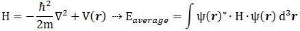
To the purists: sorry for not (always) using the hat symbol. [I explained why in that post of mine: it’s just too cumbersome.] The others 🙂 should note the following:

• E_average is also an expected value: E_av = E[E]
• The * symbol tells us to take the complex conjugate of the wavefunction.
• As for the integral, it’s an integral over some volume, so that’s what the d³r shows. Many authors use double or triple integral signs (∫∫ or ∫∫∫) to show it’s a surface or a volume integral, but that makes things look very complicated, and so I don’t that. I could also have written the integral as ∫ψ(r)*·H·ψ(r) dV, but then I’d need to explain that the dV stands for dVolume, not for any (differental) potential energy (V).
• We must normalize our wavefunction for these formulas to work, so all probabilities over the volume add up to 1.

OK. That’s the energy operator. As you can see, it’s a pretty formidable beast, but then it just reflects Schrödinger’s equation which, as I explained a couple of times already, we can interpret as an energy propagation mechanism, or an energy diffusion equation, so it is actually not that difficult to memorize the formula: if you’re able to remember Schrödinger’s equation, then you’ll also have the operator. If not… Well… Then you won’t pass your undergrad physics exam. 🙂

I already mentioned that the position operator is a much simpler beast. That’s because it’s so intimately related to our interpretation of the wavefunction. It’s the one thing you know about quantum mechanics: the absolute square of the wavefunction gives us the probability density function. So, for one-dimensional space, the position operator is just:

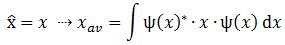
The equivalent operator for three-dimensional space is equally simple:

Note how the operator, for the one- as well as for the three-dimensional case, gets rid of time as a variable. In fact, the idea itself of an average makes abstraction of the temporal aspect. Well… Here, at least—because we’re looking at some box in space, rather than some box in spacetime. We’ll re-visit that rather particular idea of an average, and allow for averages that change with time, in a short while.

Next, we introduced the momentum operator in that post of mine. For one dimension, Feynman shows this operator is given by the following formula:

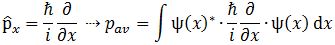
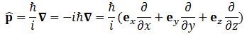
Now that does not look very simple. You might think that the ∂/∂x operator reflects our velocity operator, but… Well… No: ∂/∂t gives us a time rate of change, while ∂/∂x gives us the spatial variation. So it’s not the same. Also, that ħ/i factor is quite intriguing, isn’t it? We’ll come back to it in the next section of this post. Let me just give you the three-dimensional equivalent which, remembering that 1/i = −i, you’ll understand to be equal to the following vector operator:

Now it’s time to define the operator we wanted to talk about, i.e. the angular momentum operator.

The angular momentum operator

The formula for the angular momentum operator is remarkably simple:

Why do I call this a simple formula? Because it looks like the familiar formula of classical mechanics for the z-component of the classical angular momentum L = r × p. I must assume you know how to calculate a vector cross product. If not, check one of my many posts on vector analysis. I must also assume you remember the L = r × p formula. If not, the following animation might bring it all back. If that doesn’t help, check my post on gyroscopes. 🙂

Now, spin is a complicated phenomenon, and so, to simplify the analysis, we should think of orbital angular momentum only. This is a simplification, because electron spin is some complicated mix of intrinsic and orbital angular momentum. Hence, the angular momentum operator we’re introducing here is only the orbital angular momentum operator. However, let us not get bogged down in all of the nitty-gritty and, hence, let’s just go along with it for the time being.

I am somewhat hesitant to show you how we get that formula for our operator, but I’ll try to show you using an intuitive approach, which uses only bits and pieces of Feynman’s more detailed derivation. It will, hopefully, give you a bit of an idea of how these differential operators work. Think about a rotation of our reference frame over an infinitesimally small angle – which we’ll denote as ε – as illustrated below.

Now, the whole idea is that, because of that rotation of our reference frame, our wavefunction will look different. It’s nothing fundamental, but… Well… It’s just because we’re using a different coordinate system. Indeed, that’s where all these complicated transformation rules for amplitudes come in.  I’ve spoken about these at length when we were still discussing n-state systems. In contrast, the transformation rules for the coordinates themselves are very simple:

Now, because ε is an infinitesimally small angle, we may equate cos(θ) = cos(ε) to 1, and cos(θ) = sin(ε) to ε. Hence, x’ and y’ are then written as x’ = x + εy and y’ = y − εx, while z‘ remains z. Vice versa, we can also write the old coordinates in terms of the new ones: x = x’ − εy, y = y’ + εx, and z = z‘. That’s obvious. Now comes the difficult thing: you need to think about the two-dimensional equivalent of the simple illustration below.

If we have some function y = f(x), then we know that, for small Δx, we have the following approximation formula for f(x + Δx): f(x + Δx) ≈ f(x) + (dy/dx)·Δx. It’s the formula you saw in high school: you would then take a limit (Δx → 0), and define dy/dx as the Δy/Δx ratio for Δx → 0. You would this after re-writing the f(x + Δx) ≈ f(x) + (dy/dx)·Δx formula as:

Δy = Δf = f(x + Δx) − f(x) ≈ (dy/dx)·Δx

Now you need to substitute f for ψ, and Δx for ε. There is only one complication here: ψ is a function of two variables: x and y. In fact, it’s a function of three variables – x, y and z – but we keep z constant. So think of moving from x and y to x + εy = x + Δx and to y + Δy = y − εx. Hence, Δx = εy and Δy = −εx. It then makes sense to write Δψ as:

If you agree with that, you’ll also agree we can write something like this:

Now that implies the following formula for Δψ:

This looks great! You can see we get some sort of differential operator here, which is what we want. So the next step should be simple: we just let ε go to zero and then we’re done, right? Well… No. In quantum mechanics, it’s always a bit more complicated. But it’s logical stuff. Think of the following:

1. We will want to re-write the infinitesimally small ε angle as a fraction of i, i.e. the imaginary unit.

Huh? Yes. This little i represents many things. In this particular case, we want to look at it as a right angle. In fact, you know multiplication with i amounts to a rotation by 90 degrees. So we should replace ε by ε·i. It’s like measuring ε in natural units. However, we’re not done.

2. We should also note that Nature measures angles clockwise, rather than counter-clockwise, as evidenced by the fact that the argument of our wavefunction rotates clockwise as time goes by. So our ε is, in fact, a −ε. We will just bring the minus sign inside of the brackets to solve this issue.

Huh? Yes. Sorry. I told you this is a rather intuitive approach to getting what we want to get. 🙂

3. The third modification we’d want to make is to express ε·i as a multiple of Planck’s constant.

Huh? Yes. This is a very weird thing, but it should make sense—intuitively: we’re talking angular momentum here, and its dimension is the same as that of physical action: N·m·s. Therefore, Planck’s quantum of action (ħ = h/2π ≈ 1×10⁻³⁴ J·s ≈ 6.6×10⁻¹⁶ eV·s) naturally appears as… Well… A natural unit, or a scaling factor, I should say.

To make a long story short, we’ll want to re-write ε as −(i/ħ)·ε. However, there is a thing called mathematical consistency, and so, if we want to do such substitutions and prepare for that limit situation (ε → 0), we should re-write that Δψ equation as follows:

So now – finally! – we do have the formula we wanted to find for our angular momentum operator:

The final substitution, which yields the formula we just gave you when commencing this section, just uses the formula for the linear momentum operator in the x– and y-direction respectively. We’re done! 🙂 Finally! 

Well… No. 🙂 The question, of course, is the same as always: what does it all mean, really? That’s always a great question. 🙂 Unfortunately, the answer is rather boring: we can calculate the average angular momentum in the z-direction, using a similar integral as the one we used to get the average energy, or the average linear momentum in some direction. That’s basically it.

To compensate for that very boring answer, however, I will show you something that is far less boring. 🙂

Quantum-mechanical weirdness

I’ll shameless copy from Feynman here. He notes that many classical equations get carried over into a quantum-mechanical form (I’ll copy some of his illustrations later). But then there are some that don’t. As Feynman puts it—rather humorously: “There had better be some that don’t come out right, because if everything did, then there would be nothing different about quantum mechanics. There would be no new physics.” He then looks at the following super-obvious equation in classical mechanics:

x·p_x − p_x·x = 0

In fact, this equation is so super-obvious that it’s almost meaningless. Almost. It’s super-obvious because multiplication is commutative (for real as well for complex numbers). However, when we replace x and p_x by the position and momentum operator, we get an entirely different result. You can verify the following yourself:

This is plain weird! What does it mean? I am not sure. Feynman’s take on it is nice but leaves us in the dark on it:

He adds: “If Planck’s constant were zero, the classical and quantum results would be the same, and there would be no quantum mechanics to learn!” Hmm… What does it mean, really? Not sure. Let me make two remarks here:

1. We should not put any dot (·) between our operators, because they do not amount to multiplying one with another. We just apply operators successively. Hence, commutativity is not what we should expect.

2. Note that Feynman forgot to put the subscript in that quote. When doing the same calculations for the equivalent of the x·p_y − p_y·x expression, we do get zero, as shown below:

These equations – zero or not – are referred to as ‘commutation rules’. [Again, I should not have used any dot between x and p_y, because there is no multiplication here. It’s just a separation mark.] Let me quote Feynman on it, so the matter is dealt with:

OK. So what do we conclude? What are we talking about?

Conclusions

Some of the stuff above was really intriguing. For example, we found that the linear and angular momentum operators are differential operators in the true sense of the word. The angular momentum operator shows us what happens to the wavefunction if we rotate our reference frame over an infinitesimally small angle ε. That’s what’s captured by the formulas we’ve developed, as summarized below:

Likewise, the linear momentum operator captures what happens to the wavefunction for an infinitesimally small displacement of the reference frame, as shown by the equivalent formulas below:

What’s the interpretation for the position operator, and the energy operator? Here we are not so sure. The integrals above make sense, but these integrals are used to calculate averages values, as opposed to instantaneous values. So… Well… There is not all that much I can say about the position and energy operator right now, except… Well… We now need to explore the question of how averages could possibly change over time. Let’s do that now.

Averages that change with time

I know: you are totally quantum-mechanicked out by now. So am I. But we’re almost there. In fact, this is Feynman’s last Lecture on quantum mechanics and, hence, I think I should let the Master speak here. So just click on the link and read for yourself. It’s a really interesting chapter, as he shows us the equivalent of Newton’s Law in quantum mechanics, as well as the quantum-mechanical equivalent of other standard equations in classical mechanics. However, I need to warn you: Feynman keeps testing the limits of our intellectual absorption capacity by switching back and forth between matrix and wave mechanics. Interesting, but not easy. For example, you’ll need to remind yourself of the fact that the Hamiltonian matrix is equal to its own complex conjugate (or – because it’s a matrix – its own conjugate transpose.

Having said that, it’s all wonderful. The time rate of change of all those average values is denoted by using the over-dot notation. For example, the time rate of change of the average position is denoted by:

Once you ‘get’ that new notation, you will quickly understand the derivations. They are not easy (what derivations are in quantum mechanics?), but we get very interesting results. Nice things to play with, or think about—like this identity:

It takes a while, but you suddenly realize this is the equivalent of the classical dx/dt = v = p/m formula. 🙂

Another sweet result is the following one:

This is the quantum-mechanical equivalent of Newton’s force law: F = m·a. Huh? Yes. Think of it: the spatial derivative of the (potential) energy is the force. Now just think of the classical dp/dt = d(m·v) = m·dv/dt = m·a formula. […] Can you see it now? Isn’t this just Great Fun?

Note, however, that these formulas also show the limits of our analysis so far, because they treat m as some constant. Hence, we’ll need to relativistically correct them. But that’s complicated, and so we’ll postpone that to another day.

[…]

Well… That’s it, folks! We’re really through! This was the last of the last of Feynman’s Lectures on Physics. So we’re totally done now. Isn’t this great? What an adventure! I hope that, despite the enormous mental energy that’s required to digest all this stuff, you enjoyed it as much as I did. 🙂

Post scriptum 1: I just love Feynman but, frankly, I think he’s sometimes somewhat sloppy with terminology. In regard to what these operators really mean, we should make use of better terminology: an average is something else than an expected value. Our momentum operator, for example, as such returns an expected value – not an average momentum. We need to deepen the analysis here somewhat, but I’ll also leave that for later.

Post scriptum 2: There is something really interesting about that i·ħ or −(i/ħ) scaling factor – or whatever you want to call it – appearing in our formulas. Remember the Schrödinger equation can also be written as:

i·ħ·∂ψ/∂t = −(1/2)·(ħ²/m)∇²ψ + V·ψ = Hψ

This is interesting in light of our interpretation of the Schrödinger equation as an energy propagation mechanism. If we write Schrödinger’s equation like we write it here, then we have the energy on the right-hand side – which is time-independent. How do we interpret the left-hand side now? Well… It’s kinda simple, but we just have the time rate of change of the real and imaginary part of the wavefunction here, and the i·ħ factor then becomes a sort of unit in which we measure the time rate of change. Alternatively, you may think of ‘splitting’ Planck’s constant in two: Planck’s energy, and Planck’s time unit, and then you bring the Planck energy unit to the other side, so we’d express the energy in natural units. Likewise, the time rate of change of the components of our wavefunction would also be measured in natural time units if we’d do that.

I know this is all very abstract but, frankly, it’s crystal clear to me. This formula tells us that the energy of the particle that’s being described by the wavefunction is being carried by the oscillations of the wavefunction. In fact, the oscillations are the energy. You can play with the mass factor, by moving it to the left-hand side too, or by using Einstein’s mass-energy equivalence relation. The interpretation remains consistent.

In fact, there is something really interesting here. You know that we usually separate out the spatial and temporal part of the wavefunction, so we write: ψ(r, t) = ψ(r)·e^{−i·(E/ħ)·t}. In fact, it is quite common to refer to ψ(r) – rather than to ψ(r, t) – as the wavefunction, even if, personally, I find that quite confusing and misleading (see my page onSchrödinger’s equation). Now, we may want to think of what happens when we’d apply the energy operator to ψ(r) rather than to ψ(r, t). We may think that we’d get a time-independent value for the energy at that point in space, so energy is some function of position only, not of time. That’s an interesting thought, and we should explore it. For example, we then may think of energy as an average that changes with position—as opposed to the (average) position and momentum, which we like to think of as averages than change with time, as mentioned above. I will come back to this later – but perhaps in another post or so. Not now. The only point I want to mention here is the following: you cannot use ψ(r) in Schrödinger’s equation. Why? Well… Schrödinger’s equation is no longer valid when substituting ψ for ψ(r), because the left-hand side is always zero, as ∂ψ(r)/∂t is zero – for any r.

There is another, related, point to this observation. If you think that Schrödinger’s equation implies that the operators on both sides of Schrödinger’s equation must be equivalent (i.e. the same), you’re wrong:

i·ħ·∂/∂t ≠ H = −(1/2)·(ħ²/m)∇² + V

It’s a basic thing, really: Schrödinger’s equation is not valid for just any function. Hence, it does not work for ψ(r). Only ψ(r, t) makes it work, because… Well… Schrödinger’s equation gave us ψ(r, t)!

Some content on this page was disabled on June 16, 2020 as a result of a DMCA takedown notice from The California Institute of Technology. You can learn more about the DMCA here:

https://en.support.wordpress.com/copyright-and-the-dmca/
Some content on this page was disabled on June 16, 2020 as a result of a DMCA takedown notice from The California Institute of Technology. You can learn more about the DMCA here:

https://en.support.wordpress.com/copyright-and-the-dmca/
Some content on this page was disabled on June 16, 2020 as a result of a DMCA takedown notice from The California Institute of Technology. You can learn more about the DMCA here:

https://en.support.wordpress.com/copyright-and-the-dmca/