Quantum-mechanical operators

We climbed a mountain—step by step, post by post. 🙂 We have reached the top now, and the view is gorgeous. We understand Schrödinger’s equation, which describes how amplitudes propagate through space-time. It’s the quintessential quantum-mechanical expression. Let’s enjoy now, and deepen our understanding by introducing the concept of (quantum-mechanical) operators.

The operator concept

We’ll introduce the operator concept using Schrödinger’s equation itself and, in the process, deepen our understanding of Schrödinger’s equation a bit. You’ll remember we wrote it as:

However, you’ve probably seen it like it’s written on his bust, or on his grave, or wherever, which is as follows:

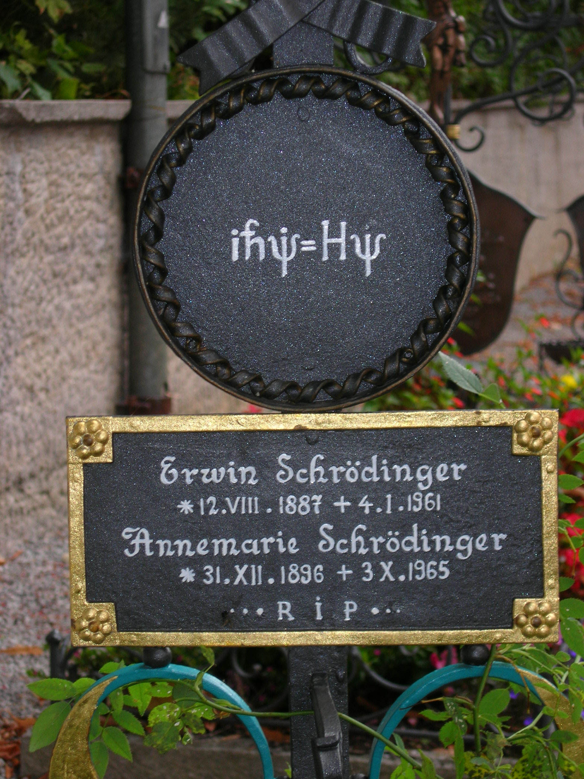
It’s the same thing, of course. The ‘over-dot’ is Newton’s notation for the time derivative. In fact, if you click on the picture above (and zoom in a bit), then you’ll see that the craftsman who made the stone grave marker, mistakenly, also carved a dot above the psi (ψ) on the right-hand side of the equation—but then someone pointed out his mistake and so the dot on the right-hand side isn’t painted. 🙂 The thing I want to talk about here, however, is the H in that expression above, which is, obviously, the following operator:

That’s a pretty monstrous operator, isn’t it? It is what it is, however: an algebraic operator (it operates on a number—albeit a complex number—unlike a matrix operator, which operates on a vector or another matrix). As you can see, it actually consists of two other (algebraic) operators:

1. The ∇² operator, which you know: it’s a differential operator. To be specific, it’s the Laplace operator, which is the divergence (∇·) of the gradient (∇) of a function: ∇² = ∇·∇ = (∂/∂x, ∂/∂y , ∂/∂z)·(∂/∂x, ∂/∂y , ∂/∂z) = ∂²/∂x²  + ∂²/∂y² + ∂²/∂z². This too operates on our complex-valued function wavefunction ψ, and yields some other complex-valued function, which we then multiply by −ħ²/2m to get the first term.
2. The V(x, y, z) ‘operator’, which—in this particular context—just means: “multiply with V”. Needless to say, V is the potential here, and so it captures the presence of external force fields. Also note that V is a real number, just like −ħ²/2m.

Let me say something about the dimensions here. On the left-hand side of Schrödinger’s equation, we have the product of ħ and a time derivative (i is just the imaginary unit, so that’s just a (complex) number). Hence, the dimension there is [J·s]/[s] (the dimension of a time derivative is something expressed per second). So the dimension of the left-hand side is joule. On the right-hand side, we’ve got two terms. The dimension of that second-order derivative (∇²ψ) is something expressed per square meter, but then we multiply it with −ħ²/2m, whose dimension is [J²·s²]/[J/(m²/s²)]. [Remember: m = E/c².] So that reduces to [J·m²]. Hence, the dimension of (−ħ²/2m)∇²ψ is joule. And the dimension of V is joule too, of course. So it all works out. In fact, now that we’re here, it may or may not be useful to remind you of that heat diffusion equation we discussed when introducing the basic concepts involved in vector analysis:

That equation illustrated the physical significance of the Laplacian. We were talking about the flow of heat in, say, a block of metal, as illustrated below. The q in the equation above is the heat per unit volume, and the h in the illustration below was the heat flow vector (so it’s got nothing to do with Planck’s constant), which depended on the material, and which we wrote as h = –κ∇T, with T the temperature, and κ (kappa) the thermal conductivity. In any case, the point is the following: the equation below illustrates the physical significance of the Laplacian. We let it operate on the temperature (i.e. a scalar function) and its product with some constant (just think of replacing κ by −ħ²/2m gives us the time derivative of q, i.e. the heat per unit volume.

In fact, we know that q is proportional to T, so if we’d choose an appropriate temperature scale – i.e. choose the zero point such that q = k·T (your physics teacher in high school would refer to k as the (volume) specific heat capacity) – then we could simple write:

∂T/∂t = (κ/k)∇²T

From a mathematical point of view, that equation is just the same as ∂ψ/∂t = –(i·ħ/2m)·∇²ψ, which is Schrödinger’s equation for V = 0. In other words, you can – and actually should – also think of Schrödinger’s equation as describing the flow of… Well… What?

Well… Not sure. I am tempted to think of something like a probability density in space, but ψ represents a (complex-valued) amplitude. Having said that, you get the idea—I hope! 🙂 If not, let me paraphrase Feynman on this:

“We can think of Schrödinger’s equation as describing the diffusion of a probability amplitude from one point to another. In fact, the equation looks something like the diffusion equation we introduced when discussing heat flow, or the spreading of a gas. But there is one main difference: the imaginary coefficient in front of the time derivative makes the behavior completely different from the ordinary diffusion such as you would have for a gas spreading out. Ordinary diffusion gives rise to real exponential solutions, whereas the solutions of Schrödinger’s equation are complex waves.”

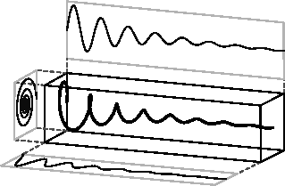
That says it all, right? 🙂 In fact, Schrödinger’s equation – as discussed here – was actually being derived when describing the motion of an electron along a line of atoms, i.e. for motion in one direction only, but you can visualize what it represents in three-dimensional space. The real exponential functions Feynman refer to exponential decay function: as the energy is spread over an ever-increasing volume, the amplitude of the wave becomes smaller and smaller. That may be the case for complex-valued exponentials as well. The key difference between a real- and complex-valued exponential decay function is that a complex exponential is a cyclical function. Now, I quickly googled to see how we could visualize that, and I like the following illustration:

The dimensional analysis of Schrödinger’s equation is also quite interesting because… Well… Think of it: that heat diffusion equation incorporates the same dimensions: temperature is a measure of the average energy of the molecules. That’s really something to think about. These differential equations are not only structurally similar but, in addition, they all seem to describe some flow of energy. That’s pretty deep stuff: it relates amplitudes to energies, so we should think in terms of Poynting vectors and all that. But… Well… I need to move on, and so I will move on—so you can re-visit this later. 🙂

Now that we’ve introduced the concept of an operator, let me say something about notations, because that’s quite confusing.

Some remarks on notation

Because it’s an operator, we should actually use the hat symbol—in line with what we did when we were discussing matrix operators: we’d distinguish the matrix (e.g. A) from its use as an operator (Â). You may or may not remember we do the same in statistics: the hat symbol is supposed to distinguish the estimator (â) – i.e. some function we use to estimate a parameter (which we usually denoted by some Greek symbol, like α) – from a specific estimate of the parameter, i.e. the value (a) we get when applying â to a specific sample or observation. However, if you remember the difference, you’ll also remember that hat symbol was quickly forgotten, because the context made it clear what was what, and so we’d just write a(x) instead of â(x). So… Well… I’ll be sloppy as well here, if only because the WordPress editor only offers very few symbols with a hat! 🙂

In any case, this discussion on the use (or not) of that hat is irrelevant. In contrast, what is relevant is to realize this algebraic operator H here is very different from that other quantum-mechanical Hamiltonian operator we discussed when dealing with a finite set of base states: that H was the Hamiltonian matrix, but used in an ‘operation’ on some state. So we have the matrix operator H, and the algebraic operator H.

Confusing?

Yes and no. First, we’ve got the context again, and so you always know whether you’re looking at continuous or discrete stuff:

1. If your ‘space’ is continuous (i.e. if states are to defined with reference to an infinite set of base states), then it’s the algebraic operator.
2. If, on the other hand, your states are defined by some finite set of discrete base states, then it’s the Hamiltonian matrix.

There’s another, more fundamental, reason why there should be no confusion. In fact, it’s the reason why physicists use the same symbol H in the first place: despite the fact that they look so different, these two operators (i.e. H the algebraic operator and H the matrix operator) are actually equivalent. Their interpretation is similar, as evidenced from the fact that both are being referred to as the energy operator in quantum physics. The only difference is that one operates on a (state) vector, while the other operates on a continuous function. It’s just the difference between matrix mechanics as opposed to wave mechanics really.

But… Well… I am sure I’ve confused you by now—and probably very much so—and so let’s start from the start. 🙂

Matrix mechanics

Let’s start with the easy thing indeed: matrix mechanics. The matrix-mechanical approach is summarized in that set of Hamiltonian equations which, by now, you know so well:

If we have n base states, then we have n equations like this: one for each i = 1, 2,… n. As for the introduction of the Hamiltonian, and the other subscript (j), just think of the description of a state:

So… Well… Because we had used i already, we had to introduce j. 🙂

Let’s think about |ψ〉. It is the state of a system, like the ground state of a hydrogen atom, or one of its many excited states. But… Well… It’s a bit of a weird term, really. It all depends on what you want to measure: when we’re thinking of the ground state, or an excited state, we’re thinking energy. That’s something else than thinking its position in space, for example. Always remember: a state is defined by a set of base states, and so those base states come with a certain perspective: when talking states, we’re only looking at some aspect of reality, really. Let’s continue with our example of energy states, however.

You know that the lifetime of a system in an excited state is usually short: some spontaneous or induced emission of a quantum of energy (i.e. a photon) will ensure that the system quickly returns to a less excited state, or to the ground state itself. However, you shouldn’t think of that here: we’re looking at stable systems here. To be clear: we’re looking at systems that have some definite energy—or so we think: it’s just because of the quantum-mechanical uncertainty that we’ll always measure some other different value. Does that make sense?

If it doesn’t… Well… Stop reading, because it’s only going to get even more confusing. Not my fault, however!

Psi-chology

The ubiquity of that ψ symbol (i.e. the Greek letter psi) is really something psi-chological 🙂 and, hence, very confusing, really. In matrix mechanics, our ψ would just denote a state of a system, like the energy of an electron (or, when there’s only one electron, our hydrogen atom). If it’s an electron, then we’d describe it by its orbital. In this regard, I found the following illustration from Wikipedia particularly helpful: the green orbitals show excitations of copper (Cu) orbitals on a CuO₂ plane. [The two big arrows just illustrate the principle of X-ray spectroscopy, so it’s an X-ray probing the structure of the material.]

So… Well… We’d write ψ as |ψ〉 just to remind ourselves we’re talking of some state of the system indeed. However, quantum physicists always want to confuse you, and so they will also use the psi symbol to denote something else: they’ll use it to denote a very particular C_i amplitude (or coefficient) in that |ψ〉 = ∑|i〉C_i formula above. To be specific, they’d replace the base states |i〉 by the continuous position variable x, and they would write the following:

C_i = ψ(i = x) = ψ(x) = C_ψ(x) = C(x) = 〈x|ψ〉

In fact, that’s just like writing:

φ(p) = 〈 mom p | ψ 〉 = 〈p|ψ〉 = C_φ(p) = C(p)

What they’re doing here, is (1) reduce the ‘system‘ to a ‘particle‘ once more (which is OK, as long as you know what you’re doing) and (2) they basically state the following:

If a particle is in some state |ψ〉, then we can associate some wavefunction ψ(x) or φ(p)—with it, and that wavefunction will represent the amplitude for the system (i.e. our particle) to be at x, or to have a momentum that’s equal to p.

So what’s wrong with that? Well… Nothing. It’s just that… Well… Why don’t they use χ(x) instead of ψ(x)? That would avoid a lot of confusion, I feel: one should not use the same symbol (psi) for the |ψ〉 state and the ψ(x) wavefunction.

Huh? Yes. Think about it. The point is: the position or the momentum, or even the energy, are properties of the system, so to speak and, therefore, it’s really confusing to use the same symbol psi (ψ) to describe (1) the state of the system, in general, versus (2) the position wavefunction, which describes… Well… Some very particular aspect (or ‘state’, if you want) of the same system (in this case: its position). There’s no such problem with φ(p), so… Well… Why don’t they use χ(x) instead of ψ(x) indeed? I have only one answer: psi-chology. 🙂

In any case, there’s nothing we can do about it and… Well… In fact, that’s what this post is about: it’s about how to describe certain properties of the system. Of course, we’re talking quantum mechanics here and, hence, uncertainty, and, therefore, we’re going to talk about the average position, energy, momentum, etcetera that’s associated with a particular state of a system, or—as we’ll keep things very simple—the properties of a ‘particle’, really. Think of an electron in some orbital, indeed! 🙂

So let’s now look at that set of Hamiltonian equations once again:

Looking at it carefully – so just look at it once again! 🙂 – and thinking about what we did when going from the discrete to the continuous setting, we can now understand we should write the following for the continuous case:

Of course, combining Schrödinger’s equation with the expression above implies the following:

Now how can we relate that integral to the expression on the right-hand side? I’ll have to disappoint you here, as it requires a lot of math to transform that integral. It requires writing H(x, x’) in terms of rather complicated functions, including – you guessed it, didn’t you? – Dirac’s delta function. Hence, I assume you’ll believe me if I say that the matrix- and wave-mechanical approaches are actually equivalent. In any case, if you’d want to check it, you can always read Feynman yourself. 🙂

Now, I wrote this post to talk about quantum-mechanical operators, so let me do that now.

Quantum-mechanical operators

You know the concept of an operator. As mentioned above, we should put a little hat (^) on top of our Hamiltonian operator, so as to distinguish it from the matrix itself. However, as mentioned above, the difference is usually quite clear from the context. Our operators were all matrices so far, and we’d write the matrix elements of, say, some operator A, as:

A_ij ≡ 〈 i | A | j 〉

The whole matrix itself, however, would usually not act on a base state but… Well… Just on some more general state ψ, to produce some new state φ, and so we’d write:

| φ 〉 = A | ψ 〉

Of course, we’d have to describe | φ 〉 in terms of the (same) set of base states and, therefore, we’d expand this expression into something like this:

You get the idea. I should just add one more thing. You know this important property of amplitudes: the 〈 ψ | φ 〉 amplitude is the complex conjugate of the 〈 φ | ψ 〉 amplitude. It’s got to do with time reversibility, because the complex conjugate of e^−iθ = e^{−i(ω·t−k·x)} is equal to e^iθ = e^{i(ω·t−k·x)}, so we’re just reversing the x- and t–direction. We write:

 〈 ψ | φ 〉 = 〈 φ | ψ 〉*

Now what happens if we want to take the complex conjugate when we insert a matrix, so when writing 〈 φ | A | ψ 〉 instead of 〈 φ | ψ 〉, this rules becomes:

〈 φ | A | ψ 〉* = 〈 ψ | A† | φ 〉

The dagger symbol denotes the conjugate transpose, so A† is an operator whose matrix elements are equal to A_ij† = A_ji*. Now, it may or may not happen that the A† matrix is actually equal to the original A matrix. In that case – and only in that case – we can write:

〈 ψ | A | φ 〉 = 〈 φ | A | ψ 〉*

We then say that A is a ‘self-adjoint’ or ‘Hermitian’ operator. That’s just a definition of a property, which the operator may or may not have—but many quantum-mechanical operators are actually Hermitian. In any case, we’re well armed now to discuss some actual operators, and we’ll start with that energy operator.

The energy operator (H)

We know the state of a system is described in terms of a set of base states. Now, our analysis of N-state systems showed we can always describe it in terms of a special set of base states, which are referred to as the states of definite energy because… Well… Because they’re associated with some definite energy. In that post, we referred to these energy levels as E_n (n = I, II,… N). We used boldface for the subscript n (so we wrote n instead of n) because of these Roman numerals. With each energy level, we could associate a base state, of definite energy indeed, that we wrote as |n〉. To make a long story short, we summarized our results as follows:

1. The energies E_I, E_II,…, E_n,…, E_N are the eigenvalues of the Hamiltonian matrix H.
2. The state vectors |n〉 that are associated with each energy E_n, i.e. the set of vectors |n〉, are the corresponding eigenstates.

We’ll be working with some more subscripts in what follows, and these Roman numerals and the boldface notation are somewhat confusing (if only because I don’t want you to think of these subscripts as vectors), we’ll just denote E_I, E_II,…, E_n,…, E_N as E₁, E₂,…, E_i,…, E_N, and we’ll number the states of definite energy accordingly, also using some Greek letter so as to clearly distinguish them from all our Latin letter symbols: we’ll write these states as: |η₁〉, |η₁〉,… |η_N〉. [If I say, ‘we’, I mean Feynman of course. You may wonder why he doesn’t write |E_i〉, or |ε_i〉. The answer is: writing |E_n〉 would cause confusion, because this state will appear in expressions like: |E_i〉E_i, so that’s the ‘product’ of a state (|E_i〉) and the associated scalar (E_i). Too confusing. As for using η (eta) instead of ε (epsilon) to denote something that’s got to do with energy… Well… I guess he wanted to keep the resemblance with the n, and then the Ancient Greek apparently did use this η letter  for a sound like ‘e‘ so… Well… Why not? Let’s get back to the lesson.]

Using these base states of definite energy, we can write the state of the system as:

|ψ〉 = ∑ |η_i〉 C_i  = ∑ |η_i〉〈η_i|ψ〉    over all i (i = 1, 2,… , N)

Now, we didn’t talk all that much about what these base states actually mean in terms of measuring something but you’ll believe if I say that, when measuring the energy of the system, we’ll always measure one or the other E₁, E₂,…, E_i,…, E_N value. We’ll never measure something in-between: it’s either–or. Now, as you know, measuring something in quantum physics is supposed to be destructive but… Well… Let us imagine we could make a thousand measurements to try to determine the average energy of the system. We’d do so by counting the number of times we measure E₁ (and of course we’d denote that number as N₁), E₂, E₃, etcetera. You’ll agree that we’d measure the average energy as:

However, measurement is destructive, and we actually know what the expected value of this ‘average’ energy will be, because we know the probabilities of finding the system in a particular base state. That probability is equal to the absolute square of that C_i coefficient above, so we can use the P_i = |C_i|² formula to write:

〈E_av〉 = ∑ P_i E_i over all i (i = 1, 2,… , N)

Note that this is a rather general formula. It’s got nothing to do with quantum mechanics: if A_i represents the possible values of some quantity A, and P_i is the probability of getting that value, then (the expected value of) the average A will also be equal to 〈A_av〉 = ∑ P_i A_i. No rocket science here! 🙂 But let’s now apply our quantum-mechanical formulas to that 〈E_av〉 = ∑ P_i E_i formula. [Oh—and I apologize for using the same angle brackets 〈 and 〉 to denote an expected value here—sorry for that! But it’s what Feynman does—and other physicists! You see: they don’t really want you to understand stuff, and so they often use very confusing symbols.] Remembering that the absolute square of a complex number equals the product of that number and its complex conjugate, we can re-write the 〈E_av〉 = ∑ P_i E_i formula as:

〈E_av〉 = ∑ P_i E_i = ∑ |C_i|² E_i = ∑ C_i*C_i E_i = ∑ C_i *C_i E_i = ∑ 〈ψ|η_i〉〈η_i|ψ〉E_i = ∑ 〈ψ|η_i〉E_i〈η_i|ψ〉 over all i

Now, you know that Dirac’s bra-ket notation allows numerous manipulations. For example, what we could do is take out that ‘common factor’ 〈ψ|, and so we may re-write that monster above as:

〈E_av〉 = 〈ψ| ∑ η_i〉E_i〈η_i|ψ〉 = 〈ψ|φ〉, with |φ〉 = ∑ |η_i〉E_i〈η_i|ψ〉 over all i

Huh? Yes. Note the difference between |ψ〉 = ∑ |η_i〉 C_i  = ∑ |η_i〉〈η_i|ψ〉 and |φ〉 = ∑ |η_i〉E_i〈η_i|ψ〉. As Feynman puts it: φ is just some ‘cooked-up‘ state which you get by taking each of the base states |η_i〉 in the amount E_i〈η_i|ψ〉 (as opposed to the 〈η_i|ψ〉 amounts we took for ψ).

I know: you’re getting tired and you wonder why we need all this stuff. Just hang in there. We’re almost done. I just need to do a few more unpleasant things, one of which is to remind you that this business of the energy states being eigenstates (and the energy levels being eigenvalues) of our Hamiltonian matrix (see my post on N-state systems) comes with a number of interesting properties, including this one:

H |η_i〉 = E_i|η_i〉 = |η_i〉E_i

Just think about what’s written here: on the left-hand side, we’re multiplying a matrix with a (base) state vector, and on the left-hand side we’re multiplying it with a scalar. So our |φ〉 = ∑ |η_i〉E_i〈η_i|ψ〉 sum now becomes:

|φ〉 = ∑ H |η_i〉〈η_i|ψ〉 over all i (i = 1, 2,… , N)

Now we can manipulate that expression some more so as to get the following:

|φ〉 = H ∑|η_i〉〈η_i|ψ〉 = H|ψ〉

Finally, we can re-combine this now with the 〈E_av〉 = 〈ψ|φ〉 equation above, and so we get the fantastic result we wanted:

〈E_av〉 = 〈 ψ | φ 〉 = 〈 ψ | H | ψ 〉

Huh? Yes! To get the average energy, you operate on |ψ〉 with H, and then you multiply the result with 〈ψ|. It’s a beautiful formula. On top of that, the new formula for the average energy is not only pretty but also useful, because now we don’t need to say anything about any particular set of base states. We don’t even have to know all of the possible energy levels. When we have to calculate the average energy of some system, we only need to be able to describe the state of that system in terms of some set of base states, and we also need to know the Hamiltonian matrix for that set, of course. But if we know that, we can calculate its average energy.

You’ll say that’s not a big deal because… Well… If you know the Hamiltonian, you know everything, so… Well… Yes. You’re right: it’s less of a big deal than it seems. Having said that, the whole development above is very interesting because of something else: we can easily generalize it for other physical measurements. I call it the ‘average value’ operator idea, but you won’t find that term in any textbook. 🙂 Let me explain the idea.

The average value operator (A)

The development above illustrates how we can relate a physical observable, like the (average) energy (E), to a quantum-mechanical operator (H). Now, the development above can easily be generalized to any observable that would be proportional to the energy. It’s perfectly reasonable, for example, to assume the angular momentum – as measured in some direction, of course, which we usually refer to as the z-direction – would be proportional to the energy, and so then it would be easy to define a new operator L_z, which we’d define as the operator of the z-component of the angular momentum L. [I know… That’s a bit of a long name but… Well… You get the idea.] So we can write:

〈L_z〉_av = 〈 ψ | L_z | ψ 〉

In fact, further generalization yields the following grand result:

If a physical observable A is related to a suitable quantum-mechanical operator Â, then the average value of A for the state | ψ 〉 is given by:

〈A〉_av = 〈 ψ |  | ψ 〉 = 〈 ψ | φ 〉 with | φ 〉 =  | ψ 〉

At this point, you may have second thoughts, and wonder: what state | ψ 〉? The answer is: it doesn’t matter. It can be any state, as long as we’re able to describe in terms of a chosen set of base states. 🙂

OK. So far, so good. The next step is to look at how this works for the continuity case.

The energy operator for wavefunctions (H)

We can start thinking about the continuous equivalent of the 〈E_av〉 = 〈ψ|H|ψ〉 expression by first expanding it. We write:

You know the continuous equivalent of a sum like this is an integral, i.e. an infinite sum. Now, because we’ve got two subscripts here (i and j), we get the following double integral:

Now, I did take my time to walk you through Feynman’s derivation of the energy operator for the discrete case, i.e. the operator when we’re dealing with matrix mechanics, but I think I can simplify my life here by just copying Feynman’s succinct development:

Done! Given a wavefunction ψ(x), we get the average energy by doing that integral above. Now, the quantity in the braces of that integral can be written as that operator we introduced when we started this post:

So now we can write that integral much more elegantly. It becomes:

〈E〉_av = ∫ ψ*(x) H ψ(x) dx

You’ll say that doesn’t look like 〈E_av〉 = 〈 ψ | H | ψ 〉! It does. Remember that 〈 ψ | = | ψ 〉*. 🙂 Done!

I should add one qualifier though: the formula above assumes our wavefunction has been normalized, so all probabilities add up to one. But that’s a minor thing. The only thing left to do now is to generalize to three dimensions. That’s easy enough. Our expression becomes a volume integral:

〈E〉_av = ∫ ψ*(r) H ψ(r) dV

Of course, dV stands for dVolume here, not for any potential energy, and, of course, once again we assume all probabilities over the volume add up to 1, so all is normalized. Done! 🙂

We’re almost done with this post. What’s left is the position and momentum operator. You may think this is going to another lengthy development but… Well… It turns out the analysis is remarkably simple. Just stay with me a few more minutes and you’ll have earned your degree. 🙂

The position operator (x)

The thing we need to solve here is really easy. Look at the illustration below as representing the probability density of some particle being at x. Think about it: what’s the average position?

Well? What? The (expected value of the) average position is just this simple integral: 〈x〉_av = ∫ x P(x) dx, over all the whole range of possible values for x. 🙂 That’s all. Of course, because P(x) = |ψ(x)|² =ψ*(x)·ψ(x), this integral now becomes:

〈x〉_av = ∫ ψ*(x) x ψ(x) dx

That looks exactly the same as 〈E〉_av = ∫ ψ*(x) H ψ(x) dx, and so we can look at x as an operator too!

Huh? Yes. It’s an extremely simple operator: it just means “multiply by x“. 🙂

I know you’re shaking your head now: is it that easy? It is. Moreover, the ‘matrix-mechanical equivalent’ is equally simple but, as it’s getting late here, I’ll refer you to Feynman for that. 🙂

The momentum operator (p_x)

Now we want to calculate the average momentum of, say, some electron. What integral would you use for that? […] Well… What? […] It’s easy: it’s the same thing as for x. We can just substitute replace x for p in that 〈x〉_av = ∫ x P(x) dx formula, so we get:

〈p〉_av = ∫ p P(p) dp, over all the whole range of possible values for p

Now, you might think the rest is equally simple, and… Well… It actually is simple but there’s one additional thing in regard to the need to normalize stuff here. You’ll remember we defined a momentum wavefunction (see my post on the Uncertainty Principle), which we wrote as:

φ(p) = 〈 mom p | ψ 〉

Now, in the mentioned post, we related this momentum wavefunction to the particle’s ψ(x) = 〈x|ψ〉 wavefunction—which we should actually refer to as the position wavefunction, but everyone just calls it the particle’s wavefunction, which is a bit of a misnomer, as you can see now: a wavefunction describes some property of the system, and so we can associate several wavefunctions with the same system, really! In any case, we noted the following there:

• The two probability density functions, φ(p) and ψ(x), look pretty much the same, but the half-width (or standard deviation) of one was inversely proportional to the half-width of the other. To be precise, we found that the constant of proportionality was equal to ħ/2, and wrote that relation as follows: σ_p = (ħ/2)/σ_x.
• We also found that, when using a regular normal distribution function for ψ(x), we’d have to normalize the probability density function by inserting a (2πσ_x²)^−1/2 in front of the exponential.

Now, it’s a bit of a complicated argument, but the upshot is that we cannot just write what we usually write, i.e. P_i = |C_i|² or P(x) = |ψ(x)|². No. We need to put a normalization factor in front, which combines the two factors I mentioned above. To be precise, we have to write:

P(p) = |〈p|ψ〉|²/(2πħ)

So… Well… Our 〈p〉_av = ∫ p P(p) dp integral can now be written as:

〈p〉_av = ∫ 〈ψ|p〉p〈p|ψ〉 dp/(2πħ)

So that integral is totally like what we found for 〈x〉_av and so… We could just leave it at that, and say we’ve solved the problem. In that sense, it is easy. However, having said that, it’s obvious we’d want some solution that’s written in terms of ψ(x), rather than in terms of φ(p), and that requires some more manipulation. I’ll refer you, once more, to Feynman for that, and I’ll just give you the result:

So… Well… I turns out that the momentum operator – which I tentatively denoted as p_x above – is not so simple as our position operator (x). Still… It’s not hugely complicated either, as we can write it as:

p_x ≡ (ħ/i)·(∂/∂x)

Of course, the purists amongst you will, once again, say that I should be more careful and put a hat wherever I’d need to put one so… Well… You’re right. I’ll wrap this all up by copying Feynman’s overview of the operators we just explained, and so he does use the fancy symbols. 🙂

Well, folks—that’s it! Off we go! You know all about quantum physics now! We just need to work ourselves through the exercises that come with Feynman’s Lectures, and then you’re ready to go and bag a degree in physics somewhere. So… Yes… That’s what I want to do now, so I’ll be silent for quite a while now. Have fun! 🙂

Some content on this page was disabled on June 16, 2020 as a result of a DMCA takedown notice from The California Institute of Technology. You can learn more about the DMCA here:

https://en.support.wordpress.com/copyright-and-the-dmca/
Some content on this page was disabled on June 16, 2020 as a result of a DMCA takedown notice from The California Institute of Technology. You can learn more about the DMCA here:

https://en.support.wordpress.com/copyright-and-the-dmca/
Some content on this page was disabled on June 16, 2020 as a result of a DMCA takedown notice from The California Institute of Technology. You can learn more about the DMCA here:

https://en.support.wordpress.com/copyright-and-the-dmca/
Some content on this page was disabled on June 16, 2020 as a result of a DMCA takedown notice from The California Institute of Technology. You can learn more about the DMCA here:

https://en.support.wordpress.com/copyright-and-the-dmca/
Some content on this page was disabled on June 16, 2020 as a result of a DMCA takedown notice from The California Institute of Technology. You can learn more about the DMCA here:

https://en.support.wordpress.com/copyright-and-the-dmca/