
In my previous post, I showed how Feynman derives Schrödinger’s equation using a historical and, therefore, quite intuitive approach. The approach was intuitive because the argument used a discrete model, so that’s stuff we are well acquainted with—like a crystal lattice, for example. However, now we’re now going to think continuity from the start. Let’s first see what changes in terms of notation.
New notations
Our C(xn, t) = 〈xn|ψ〉 now becomes C(x) = 〈x|ψ〉. This notation does not explicitly show the time dependence but then you know amplitudes like this do vary in space as well as in time. Having said that, the analysis below focuses mainly on their behavior in space, so it does make sense to not explicitly mention the time variable. It’s the usual trick: we look at how stuff behaves in space or, alternatively, in time. So we temporarily ‘forget’ about the other variable. That’s just how we work: it’s hard for our mind to think about these wavefunctions in both dimensions simultaneously although, ideally, we should do that.
Now, you also know that quantum physicists prefer to denote the wavefunction C(x) with some Greek letter: ψ (psi) or φ (phi). Feynman think it’s somewhat confusing because we use the same to denote a state itself, but I don’t agree. I think it’s pretty straightforward. In any case, we write:
ψ(x) = Cψ(x) = C(x) = 〈x|ψ〉
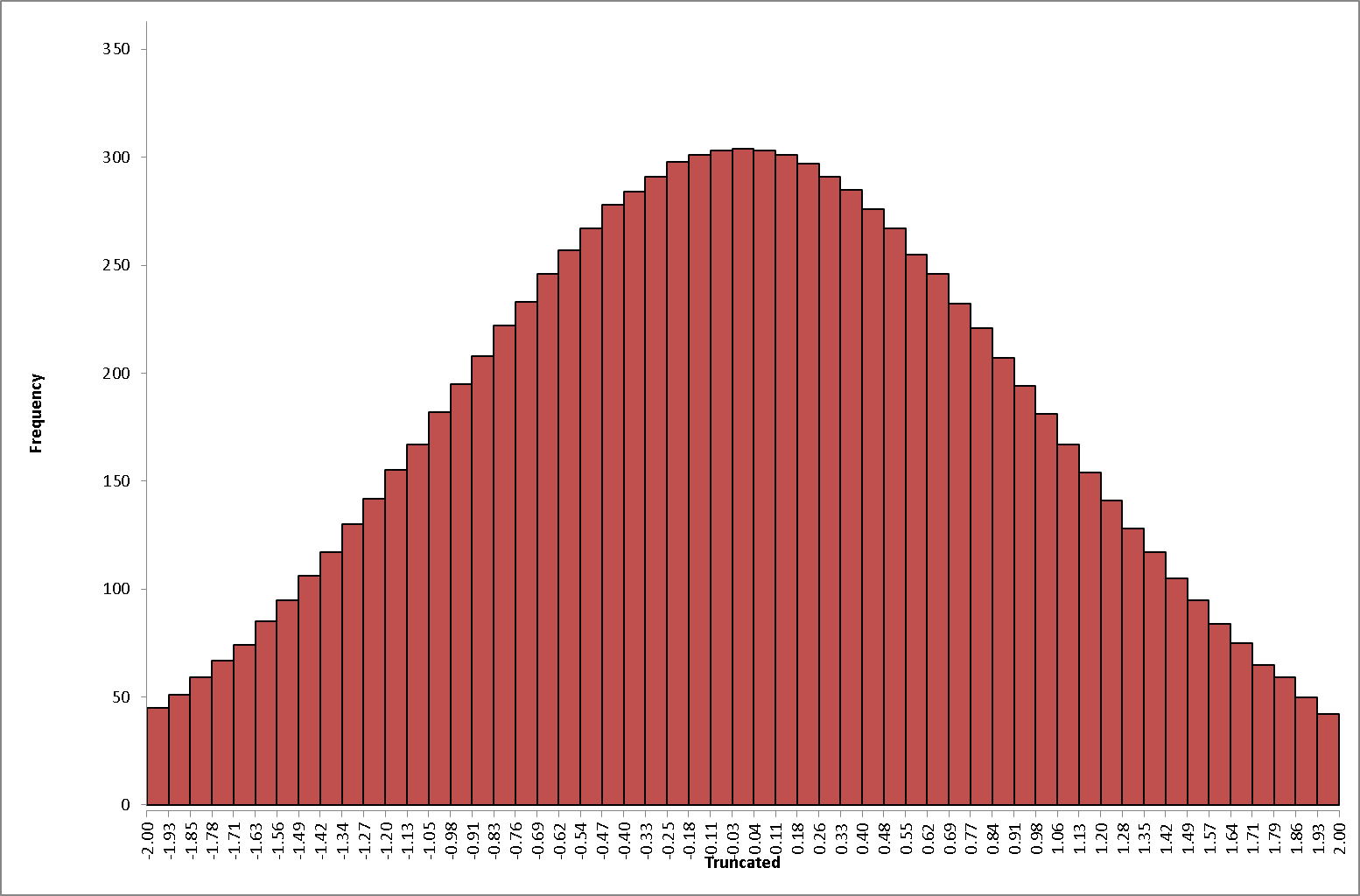
The next thing is the associated probabilities. From your high school math course, you’ll surely remember that we have two types of probability distributions: they are either discrete or, else, continuous. If they’re continuous, then our probability distribution becomes a probability density function (PDF) and, strictly speaking, we should no longer say that the probability of finding our particle at any particular point x at some time t is this or that. That probability is, strictly speaking, zero: if our variable is continuous, then our probability is defined for an interval only, and the P[x] value itself is referred to as a probability density. So we’ll look at little intervals Δx, and we can write the associated probability as:
prob (x, Δx) = |〈x|ψ〉|2Δx = |ψ(x)|2Δx
The idea is illustrated below. We just re-divide our continuous scale in little intervals and calculate the surface of some tiny elongated rectangle now. 🙂
It is also easy to see that, when moving to an infinite set of states, our 〈φ|ψ〉 = ∑〈φ|x〉〈x|ψ〉 (over all x) formula for calculating the amplitude for a particle to go from state ψ to state φ should now be written as an infinite sum, i.e. as the following integral:

Now, we know that 〈φ|x〉 = 〈x|φ〉* and, therefore, this integral can also be written as:
For example, if φ(x) = 〈x|φ〉 is equal to a simple exponential, so we can write φ(x) = a·e−iθ, then φ*(x) = 〈φ|x〉 = a·e+iθ.
With that, we’re ready for the plat de résistance, except for one thing, perhaps: we don’t look at spin here. If we’d do that, we’d have to take two sets of base sets: one for up and one for down spin—but we don’t worry about this, for the time being, that is. 🙂
The momentum wavefunction
Our wavefunction 〈x|ψ〉 varies in time as well as in space. That’s obvious. How exactly depends on the energy and the momentum: both are related and, hence, if there’s uncertainty in the momentum, there will be uncertainty in the momentum, and vice versa. Uncertainty in the momentum changes the behavior of the wavefunction in space—through the p = ħk factor in the argument of the wavefunction (θ = ω·t − k·x)—while uncertainty in the energy changes the behavior of the wavefunction in time—through the E = ħω relation. As mentioned above, we focus on the variation in space here. We’ll do so y defining a new state, which is referred to as a state of definite momentum. We’ll write it as mom p, and so now we can use the Dirac notation to write the amplitude for an electron to have a definite momentum equal to p as:
φ(p) = 〈 mom p | ψ 〉
Now, you may think that the 〈x|ψ〉 and 〈mom p|ψ〉 amplitudes should be the same because, surely, we do associate the x state with a definite momentum p, don’t we? Well… No! If we want to localize our wave ‘packet’, i.e. localize our particle, then we’re actually not going to associate it with a definite momentum. See my previous posts: we’re going to introduce some uncertainty so our wavefunction is actually a superposition of more elementary waves with slightly different (spatial) frequencies. So we should just go through the motions here and apply our integral formula to ‘unpack’ this amplitude. That goes as follows:
So, as usual, when seeing a formula like this, we should remind ourselves of what we need to solve. Here, we assume we somehow know the ψ(x) = 〈x|ψ〉 wavefunction, so the question is: what do we use for 〈 mom p | x 〉? At this point, Feynman wanders off to start a digression on normalization, which really confuses the picture. When everything is said and done, the easiest thing to do is to just jot down the formula for that 〈mom p | x〉 in the integrand and think about it for a while:
〈mom p | x〉 = e−i(p/ħ)∙x
I mean… What else could it be? This formula is very fundamental, and I am not going to try to explain it. As mentioned above, Feynman tries to ‘explain’ it by some story about probabilities and normalization, but I think his ‘explanation’ just confuses things even more. Really, what else would it be? The formula above really encapsulates what it means if we say that p and x are conjugate variables. [I can already note, of course, that symmetry implies that we can write something similar for energy and time. Indeed, we can define a state of definite energy as 〈E | ψ〉, and then ‘unpack’ it in the same way, and see that one of the two factors in the integrand would be equal to 〈E | t〉 and, of course, we’d associate a similar formula with it:
〈E | t〉 = ei(E/ħ)∙t
But let me get back to the lesson here. We’re analyzing stuff in space now, not in time. Feynman gives a simple example here. He suggests a wavefunction which has the following form:
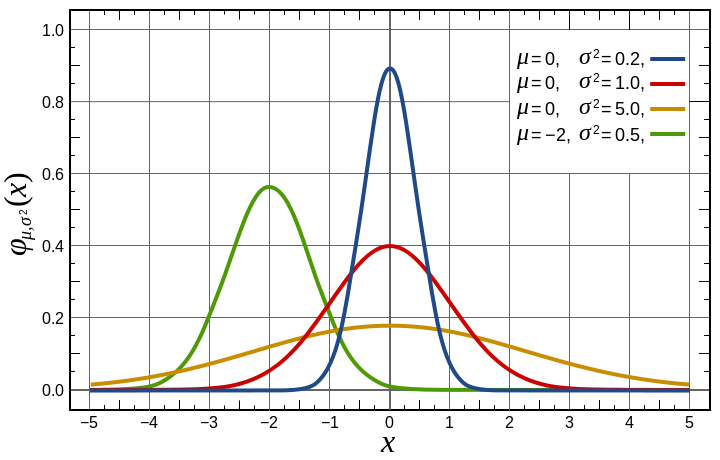
ψ(x) = K·e−x2/4σ2
The example is somewhat disingenuous because this is not a complex– but real-valued function. In fact, squaring it, and then calculating K applying the normalization condition (all probabilities have to add up to one), yields the normal probability distribution:
prob (x, Δx) = P(x)dx = (2πσ2)−1/2e−x2/2σ2dx
So that’s just the normal distribution for μ = 0, as illustrated below.
In any case, the integral we have to solve now is:
Now, I hate integrals as much as you do (probably more) and so I assume you’re also only interested in the result (if you want the detail: check it in Feynman), which we can write as:
φ(p) = (2πη2)−1/4·e−p2/4η2, with η = ħ/2σ
This formula is totally identical to the ψ(x) = (2πσ2)−1/4·e−x2/4σ2 distribution we started with, except that it’s got another sigma value, which we denoted by η (and that’s not nu but eta), with
η = ħ/2σ
Just for the record, Feynman refers to η and σ as the ‘half-width’ of the respective distributions. Mathematicians would say they’re the standard deviation. The concept are nearly the same, but not quite. In any case, that’s another thing I’ll let you find our for yourself. 🙂 The point is: η and σ are inversely proportional to each other, and the constant of proportionality is equal to ħ/2.
Now, if we take η and σ as measures of the uncertainty in p and x respectively – which is what they are, obviously ! – then we can re-write that η = ħ/2σ as ησ = ħ/2 or, better still, as the Uncertainty Principle itself:
ΔpΔx = ħ/2
You’ll say: that’s great, but we usually see the Uncertainty Principle written as:
ΔpΔx ≥ ħ/2
So where does that come from? Well… We choose a normal distribution (or the Gaussian distribution, as physicists call it), and so that yields the ΔpΔx = ħ/2 identity. If we’d chosen another one, we’d find a slightly different relation and so… Well… Let me quote Feynman here: “Interestingly enough, it is possible to prove that for any other form of a distribution in x or p, the product ΔpΔx cannot be smaller than the one we have found here, so the Gaussian distribution gives the smallest possible value for the ΔpΔx product.”
This is great. So what about the even more approximate ΔpΔx ≥ ħ formula? Where does that come from? Well… That’s more like a qualitative version of it: it basically says the minimum value of the same product is of the same order as ħ which, as you know, is pretty tiny: it’s about 0.0000000000000000000000000000000006626 J·s. 🙂 The last thing to note is its dimension: momentum is expressed in newton-second and position in meter, obviously. So the uncertainties in them are expressed in the same unit, and so the dimension of the product is N·m·s = J·s. So this dimension combines force, distance and time. That’s quite appropriate, I’d say. The ΔEΔt product obviously does the same. But… Well… That’s it, folks! I enjoyed writing this – and I cannot always say the same of other posts! So I hope you enjoyed reading it. 🙂
Some content on this page was disabled on June 16, 2020 as a result of a DMCA takedown notice from The California Institute of Technology. You can learn more about the DMCA here:
https://wordpress.com/support/copyright-and-the-dmca/
Some content on this page was disabled on June 16, 2020 as a result of a DMCA takedown notice from The California Institute of Technology. You can learn more about the DMCA here:

3 thoughts on “The Uncertainty Principle”