Diffraction and the Uncertainty Principle (I)

Pre-script (dated 26 June 2020): This post got mutilated by the removal of material by the dark force. It should be possible, however, to follow the main story line. If anything, the lack of illustrations will help you think things through for yourself. 🙂

Original post:

In his Lectures, Feynman advances the double-slit experiment with electrons as the textbook example explaining the “mystery” of quantum mechanics. It shows interference–a property of waves–of ‘particles’, electrons: they no longer behave as particles in this experiment. While it obviously illustrates “the basic peculiarities of quantum mechanics” very well, I think the dual behavior of light – as a wave and as a stream of photons – is at least as good as an illustration. And he could also have elaborated the phenomenon of electron diffraction.

Indeed, the phenomenon of diffraction–light, or an electron beam, interfering with itself as it goes through one slit only–is equally fascinating. Frankly, I think it does not get enough attention in textbooks, including Feynman’s, so that’s why I am devoting a rather long post to it here.

To be fair, Feynman does use the phenomenon of diffraction to illustrate the Uncertainty Principle, both in his Lectures as well as in that little marvel, QED: The Strange Theory of Light of Matter–a must-read for anyone who wants to understand the (probability) wave function concept without any reference to complex numbers or what have you. Let’s have a look at it: light going through a slit or circular aperture, illustrated in the left-hand image below, creates a diffraction pattern, which resembles the interference pattern created by an array of oscillators, as shown in the right-hand image.

Let’s start with the right-hand illustration, which illustrates interference, not diffraction. We have eight point sources of electromagnetic radiation here (e.g. radio waves, but it can also be higher-energy light) in an array of length L. λ is the wavelength of the radiation that is being emitted, and α is the so-called intrinsic relative phase–or, to put it simply, the phase difference. We assume α is zero here, so the array produces a maximum in the direction θ_out = 0, i.e. perpendicular to the array. There are also weaker side lobes. That’s because the distance between the array and the point where we are measuring the intensity of the emitted radiation does result in a phase difference, even if the oscillators themselves have no intrinsic phase difference.

Interference patterns can be complicated. In the set-up below, for example, we have an array of oscillators producing not just one but many maxima. In fact, the array consists of just two sources of radiation, separated by 10 wavelengths.

The explanation is fairly simple. Once again, the waves emitted by the two point sources will be in phase in the east-west (E-W) direction, and so we get a strong intensity there: four times more, in fact, than what we would get if we’d just have one point source. Indeed, the waves are perfectly in sync and, hence, add up, and the factor four is explained by the fact that the intensity, or the energy of the wave, is proportional to the square of the amplitude: 2² = 4. We get the first minimum at a small angle away (the angle from the normal is denoted by ϕ in the illustration), where the arrival times differ by 180°, and so there is destructive interference and the intensity is zero. To be precise, if we draw a line from each oscillator to a distant point and the difference Δ in the two distances is λ/2, half an oscillation, then they will be out of phase. So this first null occurs when that happens. If we move a bit further, to the point where the difference Δ is equal to λ, then the two waves will be a whole cycle out of phase, i.e. 360°, which is the same as being exactly in phase again! And so we get many maxima (and minima) indeed.

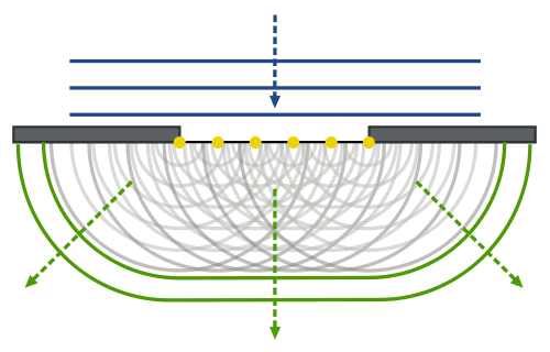
But this post should not turn into a lesson on how to construct a radio broadcasting array. The point to note is that diffraction is usually explained using this rather simple theory on interference of waves assuming that the slit itself is an array of point sources, as illustrated below (while the illustrations above were copied from Feynman’s Lectures, the ones below were taken from the Wikipedia article on diffraction). This is referred to as the Huygens-Fresnel Principle, and the math behind is summarized in Kirchhoff’s diffraction formula.

 

Now, that all looks easy enough, but the illustration above triggers an obvious question: what about the spacing between those imaginary point sources? Why do we have six in the illustration above? The relation between the length of the array and the wavelength is obviously important: we get the interference pattern that we get with those two point sources above because the distance between them is 10λ. If that distance would be different, we would get a different interference pattern. But so how does it work exactly? If we’d keep the length of the array the same (L = 10λ) but we would add more point sources, would we get the same pattern?

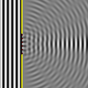
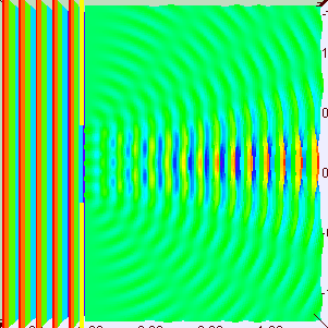
The easy answer is yes, and Kirchhoff’s formula actually assumes we have an infinite number of point sources between those two slits: every point becomes the source of a spherical wave, and the sum of these secondary waves then yields the interference pattern. The animation below shows the diffraction pattern from a slit with a width equal to five times the wavelength of the incident wave. The diffraction pattern is the same as above: one strong central beam with weaker lobes on the sides.

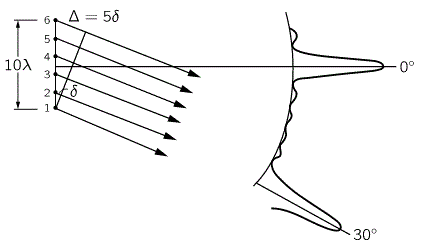
However, the truth is somewhat more complicated. The illustration below shows the interference pattern for an array of length L = 10λ–so that’s like the situation with two point sources above–but with four additional point sources to the two we had already. The intensity in the E–W direction is much higher, as we would expect. Adding six waves in phase yields a field strength that is six times as great and, hence, the intensity (which is proportional to the square of the field) is thirty-six times as great as compared to the intensity of one individual oscillator. Also, when we look at neighboring points, we find a minimum and then some more ‘bumps’, as before, but then, at an angle of 30°, we get a second beam with the same intensity as the central beam. Now, that’s something we do not see in the diffraction patterns above. So what’s going on here?

Before I answer that question, I’d like to compare with the quantum-mechanical explanation. It turns out that this question in regard to the relevance of the number of point sources also pops up in Feynman’s quantum-mechanical explanation of diffraction.

The quantum-mechanical explanation of diffraction

The illustration below (taken from Feynman’s QED, p. 55-56) presents the quantum-mechanical point of view. It is assumed that light consists of a photons, and these photons can follow any path. Each of these paths is associated with what Feynman simply refers to as an arrow, but so it’s a vector with a magnitude and a direction: in other words, it’s a complex number representing a probability amplitude.

 

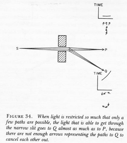
In order to get the probability for a photon to travel from the source (S) to a point (P or Q), we have to add up all the ‘arrows’ to arrive at a final ‘arrow’, and then we take its (absolute) square to get the probability. The text under each of the two illustrations above speaks for itself: when we have ‘enough’ arrows (i.e. when we allow for many neighboring paths, as in the illustration on the left), then the arrows for all of the paths from S to P will add up to one big arrow, because there is hardly any difference in time between them, while the arrows associated with the paths to Q will cancel out, because the difference in time between them is fairly large. Hence, the light will not go to Q but travel to P, i.e. in a straight line.

However, when the gap is nearly closed (so we have a slit or a small aperture), then we have only a few neighboring paths, and then the arrows to Q also add up, because there is hardly any difference in time between them too. As I am quoting from Feynman’s QED here, let me quote all of the relevant paragraph: “Of course, both final arrows are small, so there’s not much light either way through such a small hole, but the detector at Q will click almost as much as the one at P ! So when you try to squeeze light too much to make sure it’s going only in a straight line, it refuses to cooperate and begins to spread out. This is an example of the Uncertainty Principle: there is a kind of complementarity between knowledge of where the light goes between the blocks and where it goes afterwards. Precise knowledge of both is impossible.” (Feynman, QED, p. 55-56).

Feynman’s quantum-mechanical explanation is obviously more ‘true’ that the classical explanation, in the sense that it corresponds to what we know is true from all of the 20th century experiments confirming the quantum-mechanical view of reality: photons are weird ‘wavicles’ and, hence, we should indeed analyze diffraction in terms of probability amplitudes, rather than in terms of interference between waves. That being said, Feynman’s presentation is obviously somewhat more difficult to understand and, hence, the classical explanation remains appealing. In addition, Feynman’s explanation triggers a similar question as the one I had on the number of point sources. Not enough arrows !? What do we mean with that? Why can’t we have more of them? What determines their number?

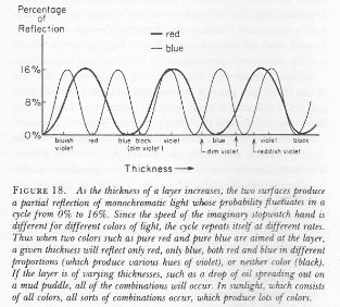
Let’s first look at their direction. Where does that come from? Feynman is a wonderful teacher here. He uses an imaginary stopwatch to determine their direction: the stopwatch starts timing at the source and stops at the destination. But all depends on the speed of the stopwatch hand of course. So how fast does it turn? Feynman is a bit vague about that but notes that “the stopwatch hand turns around faster when it times a blue photon than when it does when timing a red photon.” In other words, the speed of the stopwatch hand depends on the frequency of the light: blue light has a higher frequency (645 THz) and, hence, a shorter wavelength (465 nm) then red light, for which f = 455 THz and λ = 660 nm. Feynman uses this to explain the typical patterns of red, blue, and violet (separated by borders of black), when one shines red and blue light on a film of oil or, more generally,the phenomenon of iridescence in general, as shown below.

As for the size of the arrows, their length is obviously subject to a normalization condition, because all probabilities have to add up to 1. But what about their number? We didn’t answer that question–yet.

The answer, of course, is that the number of arrows and their size are obviously related: we associate a probability amplitude with every way an event can happen, and the (absolute) square of all these probability amplitudes has to add up to 1. Therefore, if we would identify more paths, we would have more arrows, but they would have to be smaller. The end result would be the same though: when the slit is ‘small enough’, the arrows representing the paths to Q would not cancel each other out and, hence, we’d have diffraction.

You’ll say: Hmm… OK. I sort of see the idea, but how do you explain that pattern–the central beam and the smaller side lobes, and perhaps a second beam as well? Well… You’re right to be skeptical. In order to explain the exact pattern, we need to analyze the wave functions, and that requires a mathematical approach rather than the type of intuitive approach which Feynman uses in his little QED booklet. Before we get started on that, however, let me give another example of such intuitive approach.

Diffraction and the Uncertainty Principle

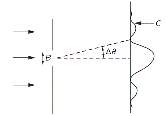
Let’s look at that very first illustration again, which I’ve copied, for your convenience, again below. Feynman uses it (III-2-2) to (a) explain the diffraction pattern which we observe when we send electrons through a slit and (b) to illustrate the Uncertainty Principle. What’s the story?

Well… Before the electrons hit the wall or enter the slit, we have more or less complete information about their momentum, but nothing on their position: we don’t know where they are exactly, and we also don’t know if they are going to hit the wall or go through the slit. So they can be anywhere. However, we do know their energy and momentum. That momentum is horizontal only, as the electron beam is normal to the wall and the slit. Hence, their vertical momentum is zero–before they hit the wall or enter the slit that is. We’ll denote their (horizontal) momentum, i.e. the momentum before they enter the slit, as p₀.

Now, if an electron happens to go through the slit, and we know because we detected it on the other side, then we know its vertical position (y) at the slit itself with considerable accuracy: that position will be the center of the slit ±B/2. So the uncertainty in position (Δy) is of the order B, so we can write: Δy = B. However, according to the Uncertainty Principle, we cannot have precise knowledge about its position and its momentum. In addition, from the diffraction pattern itself, we know that the electron acquires some vertical momentum. Indeed, some electrons just go straight, but more stray a bit away from the normal. From the interference pattern, we know that the vast majority stays within an angle Δθ, as shown in the plot. Hence, plain trigonometry allows us to write the spread in the vertical momentum p_y as p₀Δθ, with p₀ the horizontal momentum. So we have Δp_y = p₀Δθ.

Now, what is Δθ? Well… Feynman refers to the classical analysis of the phenomenon of diffraction (which I’ll reproduce in the next section) and notes, correctly, that the first minimum occurs at an angle such that the waves from one edge of the slit have to travel one wavelength farther than the waves from the other side. The geometric analysis (which, as noted, I’ll reproduce in the next section) shows that that angle is equal to the wavelength divided by the width of the slit, so we have Δθ = λ/B. So now we can write:

Δp_y = p₀Δθ = p₀λ/B

That shows that the uncertainty in regard to the vertical momentum is, indeed, inversely proportional to the uncertainty in regard to its position (Δy), which is the slit width B. But we can go one step further. The de Broglie relation relates wavelength to momentum: λ = h/p. What momentum? Well… Feynman is a bit vague on that: he equates it with the electron’s horizontal momentum, so he writes λ = h/p₀. Is this correct? Well… Yes and no. The de Broglie relation associates a wavelength with the total momentum, but then it’s obvious that most of the momentum is still horizontal, so let’s go along with this. What about the wavelength? What wavelength are we talking about here? It’s obviously the wavelength of the complex-valued wave function–the ‘probability wave’ so to say.

OK. So, what’s next? Well… Now we can write that Δp_y = p₀Δθ = p₀λ/B = p₀(h/p₀)/B. Of course, the p₀ factor vanishes and, hence, bringing B to the other side and substituting for Δy = B yields the following grand result:

Δy·Δp_y = h

Wow ! Did Feynman ‘prove’ Heisenberg’s Uncertainty Principle here?

Well… No. Not really. First, the ‘proof’ above actually assumes there’s fundamental uncertainty as to the position and momentum of a particle (so it actually assumes some uncertainty principle from the start), and then it derives it from another fundamental assumption, i.e. the de Broglie relation, which is obviously related to the Uncertainty Principle. Hence, all of the above is only an illustration of the Uncertainty Principle. It’s no proof. As far as I know, one can’t really ‘prove’ the Uncertainty Principle: it’s a fundamental assumption which, if accepted, makes our observations consistent with the theory that is based on it, i.e. quantum or wave mechanics.

Finally, note that everything that I wrote above also takes the diffraction pattern as a given and, hence, while all of the above indeed illustrates the Uncertainty Principle, it’s not an explanation of the phenomenon of diffraction as such. For such explanation, we need a rigorous mathematical analysis, and that’s a classical analysis. Let’s go for it!

Going from six to n oscillators

The mathematics involved in analyzing diffraction and/or interference are actually quite tricky. If you’re alert, then you should have noticed that I used two illustrations that both have six oscillators but that the interference pattern doesn’t match. I’ve reproduced them below. The illustration on the right-hand side has six oscillators and shows a second beam besides the central one–and, of course, there’s such beam also 30° higher, so we have (at least) three beams with the same intensity here–while the animation on the left-hand side shows only one central beam. So what’s going on here?

The answer is that, in the particular example on the left-hand side, the successive dipole radiators (i.e. the point sources) are separated by a distance of two wavelengths (2λ). In that case, it is actually possible to find an angle where the distance δ between successive dipoles is exactly one wavelength (note the little δ in the illustration, as measured from the second point source), so that the effects from all of them are in phase again. So each one is then delayed relative to the next one by 360 degrees, and so they all come back in phase, and then we have another strong beam in that direction! In this case, the other strong beam has an angle of 30 degrees as compared to the E-W line. If we would put in some more oscillators, to ensure that they are all closer than one wavelength apart, then this cannot happen. And so it’s not happening with light. 🙂 But now that we’re here, I’ll just quickly note that it’s an interesting and useful phenomenon used in diffraction gratings, but I’ll refer you to the literature on that, as I shouldn’t be bothering you with all these digressions. So let’s get back at it.

In fact, let me skip the nitty-gritty of the detailed analysis (I’ll refer you to Feynman’s Lectures for that) and just present the grand result for n oscillators, as depicted below:

This, indeed, shows the diffraction pattern we are familiar with: one strong maximum separated from successive smaller ones (note that the dotted curve magnifies the actual curve with a factor 10). The vertical axis shows the intensity, but expressed as a fraction of the maximum intensity, which is n²I₀ (I₀ is the intensity we would observe if there was only 1 oscillator). As for the horizontal axis, the variable there is ϕ really, although we re-scale the variable in order to get 1, 2, 2 etcetera for the first, second, etcetera minimum. This ϕ is the phase difference. It consists of two parts:

1. The intrinsic relative phase α, i.e. the difference in phase between one oscillator and the next: this is assumed to be zero in all of the examples of diffraction patterns above but so the mathematical analysis here is somewhat more general.
2. The phase difference which results from the fact that we are observing the array in a given direction θ from the normal. Now that‘s the interesting bit, and it’s not so difficult to show that this additional phase is equal to 2πdsinθ/λ, with d the distance between two oscillators, λ the wavelength of the radiation, and θ the angle from the normal.

In short, we write:

ϕ = α + 2πdsinθ/λ

Now, because I’ll have to use the variables below in the analysis that follows, I’ll quickly also reproduce the geometry of the set-up (all illustrations here taken from Feynman’s Lectures): 

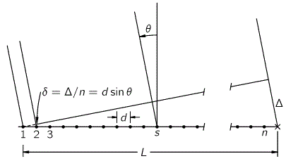
Before I proceed, please note that we assume that d is less than λ, so we only have one great maximum, and that’s the so-called zero-order beam centered at θ = 0. In order to get subsidiary great maxima (referred to as first-order, second-order, etcetera beams in the context of diffraction gratings), we must have the spacing d of the array greater than one wavelength, but so that’s not relevant for what we’re doing here, and that is to move from a discrete analysis to a continuous one.

Before we do that, let’s look at that curve again and analyze where the first minimum occurs. If we assume that α = 0 (no intrinsic relative phase), then the first minimum occurs when ϕ = 2π/n. Using the ϕ = α + 2πdsinθ/λ formula, we get 2πdsinθ/λ = 2π/n or ndsinθ = λ. What does that mean? Well, nd is the total length L of the array, so we have ndsinθ = Lsinθ = Δ = λ. What that means is that we get the first minimum when Δ is equal to one wavelength.

Now why do we get a minimum when Δ = λ? Because the contributions of the various oscillators are then uniformly distributed in phase from 0° to 360°. What we’re doing, once again, is adding arrows in order to get a resultant arrow A_R, as shown below for n = 6. At the first minimum, the arrows are going around a whole circle: we are adding equal vectors in all directions, and such a sum is zero. So when we have an angle θ such that Δ = λ, we get the first minimum. [Note that simple trigonometry rules imply that θ must be equal to λ/L, a fact which we used in that quantum-mechanical analysis of electron diffraction above.]    

What about the second minimum? Well… That occurs when ϕ = 4π/n. Using the ϕ = 2πdsinθ/λ formula again, we get 2πdsinθ/λ = 4π/n or ndsinθ = 2λ. So we get ndsinθ = Lsinθ = Δ = 2λ. So we get the second minimum at an angle θ such that Δ = 2λ. For the third minimum, we have ϕ = 6π/n. So we have 2πdsinθ/λ = 6π/n or ndsinθ = 3λ. So we get the third minimum at an angle θ such that Δ = 3λ. And so on and so on.

The point to note is that the diffraction pattern depends only on the wavelength λ and the total length L of the array, which is the width of the slit of course. Hence, we can actually extend the analysis for n going from some fixed value to infinity, and we’ll find that we will only have one great maximum with a lot of side lobes that are much and much smaller, with the minima occurring at angles such that Δ = λ, 2λ, 3λ, etcetera.

OK. What’s next? Well… Nothing. That’s it. I wanted to do a post on diffraction, and so that’s what I did. However, to wrap it all up, I’ll just include two more images from Wikipedia. The one on the left shows the diffraction pattern of a red laser beam made on a plate after passing a small circular hole in another plate. The pattern is quite clear. On the right-hand side, we have the diffraction pattern generated by ordinary white light going through a hole. In fact, it’s a computer-generated image and the gray scale intensities have been adjusted to enhance the brightness of the outer rings, because we would not be able to see them otherwise.

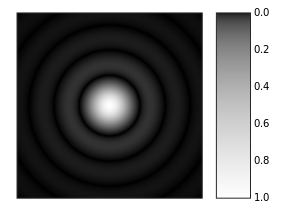
But… Didn’t I say I would write about diffraction and the Uncertainty Principle? Yes. And I admit I did not write all that much about the Uncertainty Principle above. But so I’ll do that in my next post, in which I intend to look at Heisenberg’s own illustration of the Uncertainty Principle. That example involves a good understanding of the resolving power of a lens or a microscope, and such understanding also involves some good mathematical analysis. However, as this post has become way too long already, I’ll leave that to the next post indeed. I’ll use the left-hand image above for that, so have a good look at it. In fact, let me quickly quote Wikipedia as an introduction to my next post:

The diffraction pattern resulting from a uniformly-illuminated circular aperture has a bright region in the center, known as the Airy disk which together with the series of concentric bright rings around is called the Airy pattern.

We’ll need in order to define the resolving power of a microscope, which is essential to understanding Heisenberg’s illustration of the Principle he advanced himself. But let me stop here, as it’s the topic of my next write-up indeed. This post has become way too long already. 🙂

Some content on this page was disabled on June 17, 2020 as a result of a DMCA takedown notice from Michael A. Gottlieb, Rudolf Pfeiffer, and The California Institute of Technology. You can learn more about the DMCA here:

https://en.support.wordpress.com/copyright-and-the-dmca/
Some content on this page was disabled on June 17, 2020 as a result of a DMCA takedown notice from Michael A. Gottlieb, Rudolf Pfeiffer, and The California Institute of Technology. You can learn more about the DMCA here:

https://en.support.wordpress.com/copyright-and-the-dmca/
Some content on this page was disabled on June 17, 2020 as a result of a DMCA takedown notice from Michael A. Gottlieb, Rudolf Pfeiffer, and The California Institute of Technology. You can learn more about the DMCA here:

https://en.support.wordpress.com/copyright-and-the-dmca/
Some content on this page was disabled on June 17, 2020 as a result of a DMCA takedown notice from Michael A. Gottlieb, Rudolf Pfeiffer, and The California Institute of Technology. You can learn more about the DMCA here:

https://en.support.wordpress.com/copyright-and-the-dmca/