A not so easy piece: introducing the wave equation (and the Schrödinger equation)

Pre-scriptum (dated 26 June 2020): This post did not suffer from the DMCA take-down of some material. It is, therefore, still quite readable—even if my views on these  matters have evolved quite a bit as part of my realist interpretation of QM.

Original post:

The title above refers to a previous post: An Easy Piece: Introducing the wave function.

Indeed, I may have been sloppy here and there – I hope not – and so that’s why it’s probably good to clarify that the wave function (usually represented as Ψ – the psi function) and the wave equation (Schrödinger’s equation, for example – but there are other types of wave equations as well) are two related but different concepts: wave equations are differential equations, and wave functions are their solutions.

Indeed, from a mathematical point of view, a differential equation (such as a wave equation) relates a function (such as a wave function) with its derivatives, and its solution is that function or – more generally – the set (or family) of functions that satisfies this equation. 

The function can be real-valued or complex-valued, and it can be a function involving only one variable (such as y = y(x), for example) or more (such as u = u(x, t) for example). In the first case, it’s a so-called ordinary differential equation. In the second case, the equation is referred to as a partial differential equation, even if there’s nothing ‘partial’ about it: it’s as ‘complete’ as an ordinary differential equation (the name just refers to the presence of partial derivatives in the equation). Hence, in an ordinary differential equation, we will have terms involving dy/dx and/or d²y/dx², i.e. the first and second derivative of y respectively (and/or higher-order derivatives, depending on the degree of the differential equation), while in partial differential equations, we will see terms involving ∂u/∂t and/or ∂u²/∂x² (and/or higher-order partial derivatives), with ∂ replacing d as a symbol for the derivative.

The independent variables could also be complex-valued but, in physics, they will usually be real variables (or scalars as real numbers are also being referred to – as opposed to vectors, which are nothing but two-, three- or more-dimensional numbers really). In physics, the independent variables will usually be x – or let’s use r = (x, y, z) for a change, i.e. the three-dimensional space vector – and the time variable t. An example is that wave function which we introduced in our ‘easy piece’.

Ψ(r, t) = Ae^{i(p·r – Et)ħ}

[If you read the Easy Piece, then you might object that this is not quite what I wrote there, and you are right: I wrote Ψ(r, t) = Ae^{i(p/ħ)·r – ωt)}. However, here I am just introducing the other de Broglie relation (i.e. the one relating energy and frequency): E = hf =ħω and, hence, ω = E/ħ. Just re-arrange a bit and you’ll see it’s the same.]

From a physics point of view, a differential equation represents a system subject to constraints, such as the energy conservation law (the sum of the potential and kinetic energy remains constant), and Newton’s law of course: F = d(mv)/dt. A differential equation will usually also be given with one or more initial conditions, such as the value of the function at point t = 0, i.e. the initial value of the function. To use Wikipedia’s definition: “Differential equations arise whenever a relation involving some continuously varying quantities (modeled by functions) and their rates of change in space and/or time (expressed as derivatives) is known or postulated.”

That sounds a bit more complicated, perhaps, but it means the same: once you have a good mathematical model of a physical problem, you will often end up with a differential equation representing the system you’re looking at, and then you can do all kinds of things, such as analyzing whether or not the actual system is in an equilibrium and, if not, whether it will tend to equilibrium or, if not, what the equilibrium conditions would be. But here I’ll refer to my previous posts on the topic of differential equations, because I don’t want to get into these details – as I don’t need them here.

The one thing I do need to introduce is an operator referred to as the gradient (it’s also known as the del operator, but I don’t like that word because it does not convey what it is). The gradient – denoted by ∇ – is a shorthand for the partial derivatives of our function u or Ψ with respect to space, so we write:

∇ = (∂/∂x, ∂/∂y, ∂/∂z)

You should note that, in physics, we apply the gradient only to the spatial variables, not to time. For the derivative in regard to time, we just write ∂u/∂t or ∂Ψ/∂t.

Of course, an operator means nothing until you apply it to a (real- or complex-valued) function, such as our u(x, t) or our Ψ(r, t):

∇u = ∂u/∂x and ∇Ψ = (∂Ψ/∂x, ∂Ψ/∂y, ∂Ψ/∂z)

As you can see, the gradient operator returns a vector with three components if we apply it to a real- or complex-valued function of r, and so we can do all kinds of funny things with it combining it with the scalar or vector product, or with both. Here I need to remind you that, in a vector space, we can multiply vectors using either (i) the scalar product, aka the dot product (because of the dot in its notation: a•b) or (ii) the vector product, aka as the cross product (yes, because of the cross in its notation: a×b).

So we can define a whole range of new operators using the gradient and these two products, such as the divergence and the curl of a vector field. For example, if E is the electric field vector (I am using an italic bold-type E so you should not confuse E with the energy E, which is a scalar quantity), then div E = ∇•E, and curl E =∇×E. Taking the divergence of a vector will yield some number (so that’s a scalar), while taking the curl will yield another vector. 

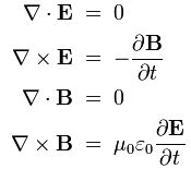
I am mentioning these operators because you will often see them. A famous example is the set of equations known as Maxwell’s equations, which integrate all of the laws of electromagnetism and from which we can derive the electromagnetic wave equation:

(1) ∇•E = ρ/ε₀ (Gauss’ law)

(2) ∇×E = –∂B/∂t (Faraday’s law)

(3) ∇•B = 0

(4) c²∇×B =  j/ε₀ +  ∂E/∂t  

I should not explain these but let me just remind you of the essentials:

1. The first equation (Gauss’ law) can be derived from the equations for Coulomb’s law and the forces acting upon a charge q in an electromagnetic field: F = q(E + v×B) – with B the magnetic field vector (F is also referred to as the Lorentz force: it’s the combined force on a charged particle caused by the electric and magnetic fields; v the velocity of the (moving) charge;  ρ the charge density (so charge is thought of as being distributed in space, rather than being packed into points, and that’s OK because our scale is not the quantum-mechanical one here); and, finally, ε₀ the electric constant (some 8.854×10⁻¹² farads per meter).
2. The second equation (Faraday’s law) gives the electric field associated with a changing magnetic field.
3. The third equation basically states that there is no such thing as a magnetic charge: there are only electric charges.
4. Finally, in the last equation, we have a vector j representing the current density: indeed, remember than magnetism only appears when (electric) charges are moving, so if there’s an electric current. As for the equation itself, well… That’s a more complicated story so I will leave that for the post scriptum.

We can do many more things: we can also take the curl of the gradient of some scalar, or the divergence of the curl of some vector (both have the interesting property that they are zero), and there are many more possible combinations – some of them useful, others not so useful. However, this is not the place to introduce differential calculus of vector fields (because that’s what it is).

The only other thing I need to mention here is what happens when we apply this gradient operator twice. Then we have an new operator ∇•∇ = ∇² which is referred to as the Laplacian. In fact, when we say ‘apply ∇ twice’, we are actually doing a dot product. Indeed, ∇ returns a vector, and so we are going to multiply this vector once again with a vector using the dot product rule: a•b = ∑a_ib_i (so we multiply the individual vector components and then add them). In the case of our functions u and Ψ, we get:

∇•(∇u) =∇•∇u = (∇•∇)u = ∇² u =∂²u/∂x²

∇•(∇Ψ) = ∇² Ψ = ∂²Ψ/∂x² + ∂²Ψ/∂y² + ∂²Ψ/∂z²

Now, you may wonder what it means to take the derivative (or partial derivative) of a complex-valued function (which is what we are doing in the case of Ψ) but don’t worry about that: a complex-valued function of one or more real variables,  such as our Ψ(x, t), can be decomposed as Ψ(x, t) =Ψ_Re(x, t) + iΨ_Im(x, t), with Ψ_Re and Ψ_Re two real-valued functions representing the real and imaginary part of Ψ(x, t) respectively. In addition, the rules for integrating complex-valued functions are, to a large extent, the same as for real-valued functions. For example, if z is a complex number, then de^z/dz = e^z and, hence, using this and other very straightforward rules, we can indeed find the partial derivatives of a function such as Ψ(r, t) = Ae^{i(p·r – Et)ħ} with respect to all the (real-valued) variables in the argument.

The electromagnetic wave equation  

OK. That’s enough math now. We are ready now to look at – and to understand – a real wave equation – I mean one that actually represents something in physics. Let’s take Maxwell’s equations as a start. To make it easy – and also to ensure that you have easy access to the full derivation – we’ll take the so-called Heaviside form of these equations:

This Heaviside form assumes a charge-free vacuum space, so there are no external forces acting upon our electromagnetic wave. There are also no other complications such as electric currents. Also, the c² (i.e. the square of the speed of light) is written here c² = 1/με, with μ and ε the so-called permeability (μ) and permittivity (ε) respectively (c₀, μ₀ and ε₀ are the values in a vacuum space: indeed, light travels slower elsewhere (e.g. in glass) – if at all).

Now, these four equations can be replaced by just two, and it’s these two equations that are referred to as the electromagnetic wave equation(s):

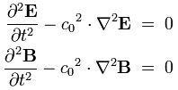
The derivation is not difficult. In fact, it’s much easier than the derivation for the Schrödinger equation which I will present in a moment. But, even if it is very short, I will just refer to Wikipedia in case you would be interested in the details (see the article on the electromagnetic wave equation). The point here is just to illustrate what is being done with these wave equations and why – not so much how. Indeed, you may wonder what we have gained with this ‘reduction’.

The answer to this very legitimate question is easy: the two equations above are second-order partial differential equations which are relatively easy to solve. In other words, we can find a general solution, i.e. a set or family of functions that satisfy the equation and, hence, can represent the wave itself. Why a set of functions? If it’s a specific wave, then there should only be one wave function, right? Right. But to narrow our general solution down to a specific solution, we will need extra information, which are referred to as initial conditions, boundary conditions or, in general, constraints. [And if these constraints are not sufficiently specific, then we may still end up with a whole bunch of possibilities, even if they narrowed down the choice.]

Let’s give an example by re-writing the above wave equation and using our function u(x, t) or, to simplify the analysis, u(x, t) – so we’re looking at a plane wave traveling in one dimension only:

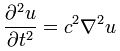
There are many functional forms for u that satisfy this equation. One of them is the following:

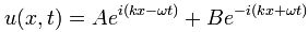
This resembles the one I introduced when presenting the de Broglie equations, except that – this time around – we are talking a real electromagnetic wave, not some probability amplitude. Another difference is that we allow a composite wave with two components: one traveling in the positive x-direction, and one traveling in the negative x-direction. Now, if you read the post in which I introduced the de Broglie wave, you will remember that these Ae^i(kx–ωt) or Be^–i(kx+ωt) waves give strange probabilities. However, because we are not looking at some probability amplitude here – so it’s not a de Broglie wave but a real wave (so we use complex number notation only because it’s convenient but, in practice, we’re only considering the real part), this functional form is quite OK.

That being said, the following functional form, representing a wave packet (aka a wave train) is also a solution (or a set of solutions better):

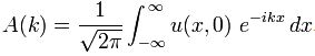
Huh? Well… Yes. If you really can’t follow here, I can only refer you to my post on Fourier analysis and Fourier transforms: I cannot reproduce that one here because that would make this post totally unreadable. We have a wave packet here, and so that’s the sum of an infinite number of component waves that interfere constructively in the region of the envelope (so that’s the location of the packet) and destructively outside. The integral is just the continuum limit of a summation of n such waves. So this integral will yield a function u with x and t as independent variables… If we know A(k) that is. Now that’s the beauty of these Fourier integrals (because that’s what this integral is). 

Indeed, in my post on Fourier transforms I also explained how these amplitudes A(k) in the equation above can be expressed as a function of u(x, t) through the inverse Fourier transform. In fact, I actually presented the Fourier transform pair Ψ(x) and Φ(p) in that post, but the logic is same – except that we’re inserting the time variable t once again (but with its value fixed at t=0):

OK, you’ll say, but where is all of this going? Be patient. We’re almost done. Let’s now introduce a specific initial condition. Let’s assume that we have the following functional form for u at time t = 0:

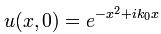
You’ll wonder where this comes from. Well… I don’t know. It’s just an example from Wikipedia. It’s random but it fits the bill: it’s a localized wave (so that’s a a wave packet) because of the very particular form of the phase (θ = –x²+ ik₀x). The point to note is that we can calculate A(k) when inserting this initial condition in the equation above, and then – finally, you’ll say – we also get a specific solution for our u(x, t) function by inserting the value for A(k) in our general solution. In short, we get:

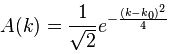
and

As mentioned above, we are actually only interested in the real part of this equation (so that’s the e with the exponent factor (note there is no i in it, so it’s just some real number) multiplied with the cosine term).

However, the example above shows how easy it is to extend the analysis to a complex-valued wave function, i.e. a wave function describing a probability amplitude. We will actually do that now for Schrödinger’s equation. [Note that the example comes from Wikipedia’s article on wave packets, and so there is a nice animation which shows how this wave packet (be it the real or imaginary part of it) travels through space. Do watch it!]

Schrödinger’s equation

Let me just write it down:

That’s it. This is the Schrödinger equation – in a somewhat simplified form but it’s OK.

[…] You’ll find that equation above either very simple or, else, very difficult depending on whether or not you understood most or nothing at all of what I wrote above it. If you understood something, then it should be fairly simple, because it hardly differs from the other wave equation.

Indeed, we have that imaginary unit (i) in front of the left term, but then you should not panic over that: when everything is said and done, we are working here with the derivative (or partial derivative) of a complex-valued function, and so it should not surprise us that we have an i here and there. It’s nothing special. In fact, we had them in the equation above too, but they just weren’t explicit. The second difference with the electromagnetic wave equation is that we have a first-order derivative of time only (in the electromagnetic wave equation we had ∂²u/∂t², so that’s a second-order derivative). Finally, we have a -1/2 factor in front of the right-hand term, instead of c². OK, so what? It’s a different thing – but that should not surprise us: when everything is said and done, it is a different wave equation because it describes something else (not an electromagnetic wave but a quantum-mechanical system).

To understand why it’s different, I’d need to give you the equivalent of Maxwell’s set of equations for quantum mechanics, and then show how this wave equation is derived from them. I could do that. The derivation is somewhat lengthier than for our electromagnetic wave equation but not all that much. The problem is that it involves some new concepts which we haven’t introduced as yet – mainly some new operators. But then we have introduced a lot of new operators already (such as the gradient and the curl and the divergence) so you might be ready for this. Well… Maybe. The treatment is a bit lengthy, and so I’d rather do in a separate post. Why? […] OK. Let me say a few things about it then. Here we go:

• These new operators involve matrix algebra. Fine, you’ll say. Let’s get on with it. Well… It’s matrix algebra with matrices with complex elements, so if we write a n×m matrix A as A = (a_ia_j), then the elements a_ia_j (i = 1, 2,… n and j = 1, 2,… m) will be complex numbers.
• That allows us to define Hermitian matrices: a Hermitian matrix is a square matrix A which is the same as the complex conjugate of its transpose.
• We can use such matrices as operators indeed: transformations acting on a column vector X to produce another column vector AX.
• Now, you’ll remember – from your course on matrix algebra with real (as opposed to complex) matrices, I hope – that we have this very particular matrix equation AX = λX which has non-trivial solutions (i.e. solutions X ≠ 0) if and only if the determinant of A-λI is equal to zero. This condition (det(A-λI) = 0) is referred to as the characteristic equation.
• This characteristic equation is a polynomial of degree n in λ and its roots are called eigenvalues or characteristic values of the matrix A. The non-trivial solutions X ≠ 0 corresponding to each eigenvalue are called eigenvectors or characteristic vectors.

Now – just in case you’re still with me – it’s quite simple: in quantum mechanics, we have the so-called Hamiltonian operator. The Hamiltonian in classical mechanics represents the total energy of the system: H = T + V (total energy H = kinetic energy T + potential energy V). Here we have got something similar but different. 🙂 The Hamiltonian operator is written as H-hat, i.e. an H with an accent circonflexe (as they say in French). Now, we need to let this Hamiltonian operator act on the wave function Ψ and if the result is proportional to the same wave function Ψ, then Ψ is a so-called stationary state, and the proportionality constant will be equal to the energy E of the state Ψ. These stationary states correspond to standing waves, or ‘orbitals’, such as in atomic orbitals or molecular orbitals. So we have:

I am sure you are no longer there but, in fact, that’s it. We’re done with the derivation. The equation above is the so-called time-independent Schrödinger equation. It’s called like that not because the wave function is time-independent (it is), but because the Hamiltonian operator is time-independent: that obviously makes sense because stationary states are associated with specific energy levels indeed. However, if we do allow the energy level to vary in time (which we should do – if only because of the uncertainty principle: there is no such thing as a fixed energy level in quantum mechanics), then we cannot use some constant for E, but we need a so-called energy operator. Fortunately, this energy operator has a remarkably simple functional form:

Now if we plug that in the equation above, we get our time-dependent Schrödinger equation:   

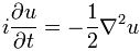
OK. You probably did not understand one iota of this but, even then, you will object that this does not resemble the equation I wrote at the very beginning: i(∂u/∂t) = (-1/2)∇²u.

You’re right, but we only need one more step for that. If we leave out potential energy (so we assume a particle moving in free space), then the Hamiltonian can be written as:

You’ll ask me how this is done but I will be short on that: the relationship between energy and momentum is being used here (and so that’s where the 2m factor in the denominator comes from). However, I won’t say more about it because this post would become way too lengthy if I would include each and every derivation and, remember, I just want to get to the result because the derivations here are not the point: I want you to understand the functional form of the wave equation only. So, using the above identity and, OK, let’s be somewhat more complete and include potential energy once again, we can write the time-dependent wave equation as:

Now, how is the equation above related to i(∂u/∂t) = (-1/2)∇²u? It’s a very simplified version of it: potential energy is, once again, assumed to be not relevant (so we’re talking a free particle again, with no external forces acting on it) but the real simplification is that we give m and ħ the value 1, so m = ħ = 1. Why?

Well… My initial idea was to do something similar as I did above and, hence, actually use a specific example with an actual functional form, just like we did for that the real-valued u(x, t) function. However, when I look at how long this post has become already, I realize I should not do that. In fact, I would just copy an example from somewhere else – probably Wikipedia once again, if only because their examples are usually nicely illustrated with graphs (and often animated graphs). So let me just refer you here to the other example given in the Wikipedia article on wave packets: that example uses that simplified i(∂u/∂t) = (-1/2)∇²u equation indeed. It actually uses the same initial condition:

However, because the wave equation is different, the wave packet behaves differently. It’s a so-called dispersive wave packet: it delocalizes. Its width increases over time and so, after a while, it just vanishes because it diffuses all over space. So there’s a solution to the wave equation, given this initial condition, but it’s just not stable – as a description of some particle that is (from a mathematical point of view – or even a physical point of view – there is no issue).

In any case, this probably all sounds like Chinese – or Greek if you understand Chinese :-). I actually haven’t worked with these Hermitian operators yet, and so it’s pretty shaky territory for me myself. However, I felt like I had picked up enough math and physics on this long and winding Road to Reality (I don’t think I am even halfway) to give it a try. I hope I succeeded in passing the message, which I’ll summarize as follows:

1. Schrödinger’s equation is just like any other differential equation used in physics, in the sense that it represents a system subject to constraints, such as the relationship between energy and momentum.
2. It will have many general solutions. In other words, the wave function – which describes a probability amplitude as a function in space and time – will have many general solutions, and a specific solution will depend on the initial conditions.
3. The solution(s) can represent stationary states, but not necessary so: a wave (or a wave packet) can be non-dispersive or dispersive. However, when we plug the wave function into the wave equation, it will satisfy that equation.

That’s neither spectacular nor difficult, is it? But, perhaps, it helps you to ‘understand’ wave equations, including the Schrödinger equation. But what is understanding? Dirac once famously said: “I consider that I understand an equation when I can predict the properties of its solutions, without actually solving it.”

Hmm… I am not quite there yet, but I am sure some more practice with it will help. 🙂

Post scriptum: On Maxwell’s equations

First, we should say something more about these two other operators which I introduced above: the divergence and the curl. First on the divergence.

The divergence of a field vector E (or B) at some point r represents the so-called flux of E, i.e. the ‘flow’ of E per unit volume. So flux and divergence both deal with the ‘flow’ of electric field lines away from (positive) charges. [The ‘away from’ is from positive charges indeed – as per the convention: Maxwell himself used the term ‘convergence’ to describe flow towards negative charges, but so his ‘convention’ did not survive. Too bad, because I think convergence would be much easier to remember.]

So if we write that ∇•E = ρ/ε₀, then it means that we have some constant flux of E because of some (fixed) distribution of charges.

Now, we already mentioned that equation (2) in Maxwell’s set meant that there is no such thing as a ‘magnetic’ charge: indeed, ∇•B = 0 means there is no magnetic flux. But, of course, magnetic fields do exist, don’t they? They do. A current in a wire, for example, i.e. a bunch of steadily moving electric charges, will induce a magnetic field according to Ampère’s law, which is part of equation (4) in Maxwell’s set: c²∇×B =  j/ε₀, with j representing the current density and ε₀ the electric constant.

Now, at this point, we have this curl: ∇×B. Just like divergence (or convergence as Maxwell called it – but then with the sign reversed), curl also means something in physics: it’s the amount of ‘rotation’, or ‘circulation’ as Feynman calls it, around some loop.

So, to summarize the above, we have (1) flux (divergence) and (2) circulation (curl) and, of course, the two must be related. And, while we do not have any magnetic charges and, hence, no flux for B, the current in that wire will cause some circulation of B, and so we do have a magnetic field. However, that magnetic field will be static, i.e. it will not change. Hence, the time derivative ∂B/∂t will be zero and, hence, from equation (2) we get that ∇×E = 0, so our electric field will be static too. The time derivative ∂E/∂t which appears in equation (4) also disappears and we just have c²∇×B =  j/ε₀. This situation – of a constant magnetic and electric field – is described as electrostatics and magnetostatics respectively. It implies a neat separation of the four equations, and it makes magnetism and electricity appear as distinct phenomena. Indeed, as long as charges and currents are static, we have:

[I] Electrostatics: (1) ∇•E = ρ/ε₀ and (2) ∇×E = 0

[II] Magnetostatics: (3) c²∇×B =  j/ε₀ and (4) ∇•B = 0

The first two equations describe a vector field with zero curl and a given divergence (i.e. the electric field) while the third and fourth equations second describe a seemingly separate vector field with a given curl but zero divergence. Now, I am not writing this post scriptum to reproduce Feynman’s Lectures on Electromagnetism, and so I won’t say much more about this. I just want to note two points:

1. The first point to note is that factor c² in the c²∇×B =  j/ε₀ equation. That’s something which you don’t have in the ∇•E = ρ/ε₀ equation. Of course, you’ll say: So what? Well… It’s weird. And if you bring it to the other side of the equation, it becomes clear that you need an awful lot of current for a tiny little bit of magnetic circulation (because you’re dividing by c²  , so that’s a factor 9 with 16 zeroes after it (9×10¹⁶):  an awfully big number in other words). Truth be said, it reveals something very deep. Hmm? Take a wild guess. […] Relativity perhaps? Well… Yes!

It’s obvious that we buried v somewhere in this equation, the velocity of the moving charges. But then it’s part of j of course: the rate at which charge flows through a unit area per second. But – Hey! – velocity as compared to what? What’s the frame of reference? The frame of reference is us obviously or – somewhat less subjective – the stationary charges determining the electric field according to equation (1) in the set above: ∇•E = ρ/ε₀. But so here we can ask the same question: stationary in what reference frame? As compared to the moving charges? Hmm… But so how does it work with relativity? I won’t copy Feynman’s 13th Lecture here, but so, in that lecture, he analyzes what happens to the electric and magnetic force when we look at the scene from another coordinate system – let’s say one that moves parallel to the wire at the same speed as the moving electrons, so – because of our new reference frame – the ‘moving electrons’ now appear to have no speed at all but, of course, our stationary charges will now seem to move.

What Feynman finds – and his calculations are very easy and straightforward – is that, while we will obviously insert different input values into Maxwell’s set of equations and, hence, get different values for the E and B fields, the actual physical effect – i.e. the final Lorentz force on a (charged) particle – will be the same. To be very specific, in a coordinate system at rest with respect to the wire (so we see charges move in the wire), we find a ‘magnetic’ force indeed, but in a coordinate system moving at the same speed of those charges, we will find an ‘electric’ force only. And from yet another reference frame, we will find a mixture of E and B fields. However, the physical result is the same: there is only one combined force in the end – the Lorentz force F = q(E + v×B) – and it’s always the same, regardless of the reference frame (inertial or moving at whatever speed – relativistic (i.e. close to c) or not).

In other words, Maxwell’s description of electromagnetism is invariant or, to say exactly the same in yet other words, electricity and magnetism taken together are consistent with relativity: they are part of one physical phenomenon: the electromagnetic interaction between (charged) particles. So electric and magnetic fields appear in different ‘mixtures’ if we change our frame of reference, and so that’s why magnetism is often described as a ‘relativistic’ effect – although that’s not very accurate. However, it does explain that c² factor in the equation for the curl of B. [How exactly? Well… If you’re smart enough to ask that kind of question, you will be smart enough to find the derivation on the Web. :-)]

Note: Don’t think we’re talking astronomical speeds here when comparing the two reference frames. It would also work for astronomical speeds but, in this case, we are talking the speed of the electrons moving through a wire. Now, the so-called drift velocity of electrons – which is the one we have to use here – in a copper wire of radius 1 mm carrying a steady current of 3 Amps is only about 1 m per hour! So the relativistic effect is tiny  – but still measurable !

2. The second thing I want to note is that  Maxwell’s set of equations with non-zero time derivatives for E and B clearly show that it’s changing electric and magnetic fields that sort of create each other, and it’s this that’s behind electromagnetic waves moving through space without losing energy. They just travel on and on. The math behind this is beautiful (and the animations in the related Wikipedia articles are equally beautiful – and probably easier to understand than the equations), but that’s stuff for another post. As the electric field changes, it induces a magnetic field, which then induces a new electric field, etc., allowing the wave to propagate itself through space. I should also note here that the energy is in the field and so, when electromagnetic waves, such as light, or radiowaves, travel through space, they carry their energy with them.

Let me be fully complete here, and note that there’s energy in electrostatic fields as well, and the formula for it is remarkably beautiful. The total (electrostatic) energy U in an electrostatic field generated by charges located within some finite distance is equal to:

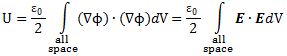
This equation introduces the electrostatic potential. This is a scalar field Φ from which we can derive the electric field vector just by applying the gradient operator. In fact, all curl-free fields (such as the electric field in this case) can be written as the gradient of some scalar field. That’s a universal truth. See how beautiful math is? 🙂