The energy of fields and the Poynting vector

For some reason, I always thought that Poynting was a Russian physicist, like Minkowski. He wasn’t. I just looked it up. Poynting was an Englishman, born near Manchester, and he teached in Birmingham. I should have known. Poynting is a very English name, isn’t it? My confusion probably stems from the fact that it was some Russian physicist, Nikolay Umov, who first proposed the basic concepts we are going to discuss here, i.e. the speed and direction of energy itself, or its movement. And as I am double-checking, I just learned that Hermann Minkowski is generally considered to be German-Jewish, not Russian. Makes sense. With Einstein and all that. His personal life story is actually quite interesting. You should check it out. 🙂

Let’s go for it. We’ve done a few posts on the energy in the fields already, but all in the contexts of electrostatics. Let me first walk you through the ideas we presented there.

The basic concepts: force, work, energy and potential

1. A charge q causes an electric field E, and E‘s magnitude E is a simple function of the charge (q) and its distance (r) from the point that we’re looking at, which we usually write as P = (x, y, z). Of course, the origin of our reference frame here is q. The formula is the simple inverse-square law that you (should) know: E ∼ q/r², and the proportionality constant is just Coulomb’s constant, which I think you wrote as k_e in your high-school days and which, as you know, is there so as to make sure the units come out alright. So we could just write E = k_e·q/r². However, just to make sure it does not look like a piece of cake 🙂 physicists write the proportionality constant as 1/4πε₀, so we get:

Now, the field is the force on any unit charge (+1) we’d bring to P. This led us to think of energy, potential energy, because… Well… You know: energy is measured by work, so that’s some force acting over some distance. The potential energy of a charge increases if we move it against the field, so we wrote:

Well… We actually gave the formula below in that post, so that’s the work done per unit charge. To interpret it, you just need to remember that F = qE, which is equivalent to saying that E is the force per unit charge.

As for the F•ds or E•ds product in the integrals, that’s a vector dot product, which we need because it’s only the tangential component of the force that’s doing work, as evidenced by the formula F•ds = |F|·|ds|·cosθ = F_t·ds, and as depicted below.

Now, this allowed us to describe the field in terms of the (electric) potential Φ and the potential differences between two points, like the points a and b in the integral above. We have to chose some reference point, of course, some P₀ defining zero potential, which is usually infinitely far away. So we wrote our formula for the work that’s being done on a unit charge, i.e. W(unit) as:

2. The world is full of charges, of course, and so we need to add all of their fields. But so now you need a bit of imagination. Let’s reconstruct the world by moving all charges out, and then we bring them back one by one. So we take q₁ now, and we bring it back into the now-empty world. Now that does not require any energy, because there’s no field to start with. However, when we take our second charge q₂, we will be doing work as we move it against the field or, if it’s an opposite charge, we’ll be taking energy out of the field. Huh? Yes. Think about it. All is symmetric. Just to make sure you’re comfortable with every step we take, let me jot down the formula for the force that’s involved. It’s just the Coulomb force of course:

F₁ is the force on charge q₁, and F₂ is the force on charge q₂. Now, q₁ and q₂. may attract or repel each other but the forces will always be equal and opposite. The e₁₂ vector makes sure the directions and signs come out alright, as it’s the unit vector from q₂ to q₁ (not from q₁ to q₂, as you might expect when looking at the order of the indices). So we would need to integrate this for r going from infinity to… Well… The distance between q₁ and q₂ – wherever they end up as we put them back into the world – so that’s what’s denoted by r₁₂. Now I hate integrals too, but this is an easy one. Just note that ∫ r⁻²dr = 1/r and you’ll be able to figure out that what I’ll write now makes sense (if not, I’ll do a similar integral in a moment): the work done in bringing two charges together from a large distance (infinity) is equal to:

So now we should bring in q₃ and then q₄, of course. That’s easy enough. Bringing the first two charges into that world we had emptied took a lot of time, but now we can automate processes. Trust me: we’ll be done in no time. 🙂 We just need to sum over all of the pairs of charges q_i and q_j. So we write the total electrostatic energy U as the sum of the energies of all possible pairs of charges:

Huh? Can we do that? I mean… Every new charge that we’re bringing in here changes the field, doesn’t it? It does. But it’s the magic of the superposition principle at work here. Our third charge q₃ is associated with two pairs in this formula. Think of it: we’ve got the q₁q₃ and the q₂q₃ combination, indeed. Likewise, our fourh charge q₄ is to be paired up with three charges now: q₁, q₁ and q₃. This formula takes care of it, and the ‘all pairs’ mention under the summation sign (Σ) reminds us we should watch we don’t double-count pairs: the q₁q₃ and q₃q₁ combination, for example, count for one pair only, obviously. So, yes, we write ‘all pairs’ instead of the usual i, j subscripts. But then, yes, this formula takes care of it. We’re done!

Well… Not really, of course. We’ve still got some way to go before I can introduce the Poynting vector. 🙂 However, to make sure you ‘get’ the energy formula above, let me insert an extremely simple diagram so you’ve got a bit of a visual of what we’re talking about.

3. Now, let’s take a step back. We just calculated the (potential) energy of the world (U), which is great. But perhaps we should also be interested in the world’s potential Φ, rather than its potential energy U. Why? Well, we’ll want to know what happens when we bring yet another charge in—from outer space or so. 🙂 And so then it’s easier to know the world’s potential, rather than its energy, because we can calculate the field from it using the E = −∇Φ formula. So let’s de- and re-construct the world once again 🙂 but now we’ll look at what happens with the field and the potential.

We know our first charge created a field with a field strength we calculated as:

So, when bringing in our second charge, we can use our Φ(P) integral to calculate the potential:

[Let me make a note here, just for the record. You probably think I am being pretty childish when talking about my re-construction of the world in terms of bringing all charges out and then back in again but, believe me, there will be a lot of confusion when we’ll start talking about the energy of one charge, and that confusion can be avoided, to a large extent, when you realize that the idea (I mean the concept itself, really—not its formula) of a potential involves two charges really. Just remember: it’s the first charge that causes the field (and, of course, any charge causes a field), but calculating a potential only makes sense when we’re talking some other charge. Just make a mental note of it. You’ll be grateful to me later.]

Let’s now combine the integral and the formula for E above. Because you hate integrals as much as I do, I’ll spell it out: the antiderivative of the Φ(P) integral is ∫ q/(4πε₀r²)·dr. Now, let’s bring q/4πε₀ out for a while so we can focus on solving ∫(1/r²)dr. Now, ∫(1/r²)dr is equal to –1/r + k, and so the whole antiderivative is –q/4πε₀r + k. Now, we integrate from r = ∞ to r, and so the definite integral is [–q/(4πε₀)]·[1/∞ − 1/r] = [–q/(4πε₀)]·[0 − 1/r] = q/(4πε₀r). Let me present this somewhat nicer:

You’ll say: so what? Well… We’re done! The only thing we need to do now is add up the potentials of all of the charges in the world. So the formula for the potential Φ at a point which we’ll simply refer to as point 1, is:

Note that our index j starts at 2, otherwise it doesn’t make sense: we’d have a division by zero for the q₁/r₁₁ term. Again, it’s an obvious remark, but not thinking about it can cause a lot of confusion down the line.

4. Now, I am very sorry but I have to inform you that we’ll be talking charge densities and all that shortly, rather than discrete charges, so I have to give you the continuum version of this formula, i.e. the formula we’ll use when we’ve got charge densities rather than individual charges. That sum above then becomes an infinite sum (i.e. an integral), and q_j becomes a variable which we write as ρ(2). [That’s totally in line with our index j starts at 2, rather than from 1.] We get:

Just look at this integral, and try to understand it: we’re integrating over all of space – so we’re integrating the whole world, really 🙂 – and the ρ(2)·dV₂ product in the integral is just the charge of an infinitesimally small volume of our world. So the whole integral is just the (infinite) sum of the contributions to the potential (at point 1) of all (infinitesimally small) charges that are around indeed. Now, there’s something funny here. It’s just a mathematical thing: we don’t need to worry about double-counting here. Why? We’re not having products of volumes here. Just make a mental note of it because it will be different in a moment.

Now we’re going to look at the continuum version for our energy formula indeed. Which energy formula? That electrostatic energy formula, which said that the total electrostatic energy U as the sum of the energies of all possible pairs of charges:

Its continuum version is the following monster:

Hmm… What kind of integral is that? We’ve got two variables here: dV₂ and dV₁. Yes. And we’ve also got a 1/2 factor now, because we do not want to double-count and, unfortunately, there is no convenient way of writing an integral like this that keeps track of the pairs. It’s a so-called double integral, but I’ll let you look up the math yourself. In any case, we can simplify this integral so you don’t need to worry about it too much. How do we simplify it? Well… Just look at that integral we got for Φ(1): we calculated the potential at point 1 by integrating the ρ(2)·dV₂ product over all of space, so the integral above can be written as:

But so this integral integrates the ρ(1)·Φ(1)·dV₁ product over all of space, so that’s over all points in space. So we can just drop the index and write the whole thing as the integral of ρ·Φ·dV over all of space:

5. It’s time for the hat-trick now. The equation above is mathematically equivalent to the following equation:

Huh? Yes. Let me make two remarks here. First on the math, the E = −∇Φ formula allows you to the integrand of the integral above as E•E = (−∇Φ)•(−∇Φ) = (∇Φ)•(∇Φ). And then you may or may not remember that, when substituting E = −∇Φ in Maxwell’s first equation (∇•E = ρ/ε₀), we got the following equality: ρ = ε₀·∇•(∇Φ) = ε₀·∇²Φ, so we can write ρΦ as ε₀·Φ·∇²Φ. However, that still doesn’t show the two integrals are the same thing. The proof is actually rather involved, and so I’ll refer to that post I referred to, so you can check the proof there.

The second remark is much more fundamental. The two integrals are mathematically equivalent, but are they also physically? What do I mean with that? Well… Look at it. The second integral implies that we can look at (ε₀/2)·E•E = ε₀E²/2 as an energy density, which we’ll denote by u, so we write:

Just to make sure you ‘get’ what we’re talking about here: u is the energy density in the little cube dV in the rather simplistic (and, therefore, extremely useful) illustration below (which, just like most of what I write above, I got from Feynman).

Now the question: what is the reality of that formula? Indeed, what we did when calculating U amounted to calculating the Universe with some number U – and that’s kinda nice, of course! – but then what? Is u = ε₀E²/2 anything real? Well… That’s what this post is about. So we’re finished with the introduction now. 🙂

Energy density and energy flow in electrodynamics

Before giving you any more formulas, let me answer the question: there is no doubt, in the classical theory of electromagnetism at least, that the energy density u is something very real. It has to be because of the charge conservation law. Charges cannot just disappear in space, to then re-appear somewhere else. The charge conservation law is written as ∇•j = −∂ρ/∂t, and that makes it clear it’s a local conservation law. Therefore, charges can only disappear and re-appear through some current. We write dQ₁/dt = ∫ (j•n)·da = −dQ₂/dt, and here’s the simple illustration that comes with it:

So we do not allow for any ‘non-local’ interactions here! Therefore, we say that, if energy goes away from a region, it’s because it flows away through the boundaries of that region. So that’s what the Poynting formulas are all about, and so I want to be clear on that from the outset.

Now, to get going with the discussion, I need to give you the formula for the energy density in electrodynamics. Its shape won’t surprise you:

However, it’s just like the electrostatic formula: it takes quite a bit of juggling to get this from our electrodynamic equations, so, if you want to see how it’s done, I’ll refer you to Feynman. Indeed, I feel the derivation doesn’t matter all that much, because the formula itself is very intuitive: it’s really the thing everyone knows about a wave, electromagnetic or not: the energy in it is proportional to the square of its amplitude, and so that’s E•E = E² and B•B = B². Now, you also know that the magnitude of B is 1/c of that of E, so cB = E, and so that explains the extra c² factor in the second term.

The second formula is also very intuitive. Let me write it down:

Just look at it: u is the energy density, so that’s the amount of energy per unit volume at a given point, and so whatever flows out of that point must represent its time rate of change. As for the –∇•S expression… Well… Sorry, I can’t keep re-explaining things: the ∇• operator is the divergence, and so it give us the magnitude of a (vector) field’s source or sink at a given point. ∇•C is a scalar, and if it’s positive in a region, then that region is a source. Conversely, if it’s negative, then it’s a sink. To be precise, the divergence represents the volume density of the outward flux of a vector field from an infinitesimal volume around a given point. So, in this case, it gives us the volume density of the flux of S. As you can see, the formula has exactly the same shape as ∇•j = −∂ρ/∂t.

So what is S? Well… Think about the more general formula for the flux out of some closed surface, which we get from integrating over the volume enclosed. It’s just Gauss’ Theorem:

Just replace C by E, and think about what it meant: the flux of E was the field strength multiplied by the surface area, so it was the total flow of E. Likewise, S represents the flow of (field) energy. Let me repeat this, because it’s an important result:

S represents the flow of field energy.

Huh? What flow? Per unit area? Per second? How do you define such ‘flow’? Good question. Let’s do a dimensional analysis:

1. E is measured in newton per coulomb, so [E•E] = [E²] = N²/C².
2. B is measured in (N/C)/(m/s). [Huh? Well… Yes. I explained that a couple of times already. Just check it in my introduction to electric circuits.] So we get [B•B] = [B²] = (N²/C²)·(s²/m²) but the dimension of our c² factor is (m²/s²) so we’re left with N²/C². That’s nice, because we need to add in the same units.
3. Now we need to look at ε₀. That constant usually ‘fixes’ our units, but can we trust it to do the same now? Let’s see… One of the many ways in which we can express its dimension is [ε₀] = C²/(N·m²), so if we multiply that with N²/C², we find that u is expressed in N/m². Wow! That’s kinda neat. Why? Well… Just multiply with m/m and its dimension becomes N·m/m³ = J/m³, so that’s  joule per cubic meter, so… Yes: u has got the right unit for something that’s supposed to measure energy density!
4. OK. Now, we take the time rate of change of u, and so both the right and left of our ∂u/∂t = −∇•S formula are expressed in (J/m³)/s, which means that the dimension of S itself must be J/(m²·s). Just check it by writing it all out: ∇•S = ∂S_x/∂x + ∂S_y/∂x + ∂S_z/∂z, and so that’s something per meter so, to get the dimension of S itself, we need to go from cubic meter to square meter. Done! Let me highlight the grand result:

S is the energy flow per unit area and per second.

Now we’ve got its magnitude and its dimension, but what is its direction? Indeed, we’ve been writing S as a vector, but… Well… What’s its direction indeed?

Well… Hmm… I referred you to Feynman for that derivation of that u = ε₀E²/2 + ε₀c²B²/2 formula energy for u, and so the direction of S – I should actually say, its complete definition – comes out of that derivation as well. So… Well… I think you should just believe what I’ll be writing here for S:

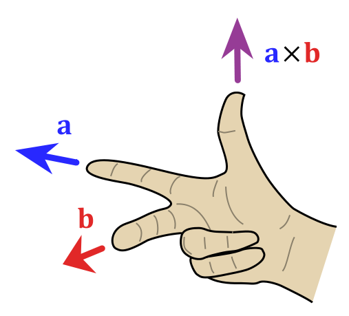
So it’s the vector cross product of E and B with ε₀c² thrown in. It’s a simple formula really, and because I didn’t drag you through the whole argument, you should just quickly do a dimensional analysis again—just to make sure I am not talking too much nonsense. 🙂 So what’s the direction? Well… You just need to apply the usual right-hand rule:

OK. We’re done! This S vector, which – let me repeat it – represents the energy flow per unit area and per second, is what is referred to as Poynting’s vector, and it’s a most remarkable thing, as I’ll show now. Let’s think about the implications of this thing.

Poynting’s vector in electrodynamics

The S vector is actually quite similar to the heat flow vector h, which we presented when discussing vector analysis and vector operators. The heat flow out of a surface element da is the area times the component of h perpendicular to da, so that’s (h•n)·da = h_n·da. Likewise, we can write (S•n)·da = S_n·da. The units of S and h are also the same: joule per second and per square meter or, using the definition of the watt (1 W = 1 J/s), in watt per square meter. In fact, if you google a bit, you’ll find that both h and S are referred to as a flux density:

1. The heat flow vector h is the heat flux density vector, from which we get the heat flux through an area through the (h•n)·da = h_n·da product.
2. The energy flow S is the energy flux density vector, from which we get the energy flux through the (S•n)·da = S_n·da product.

The big difference, of course, is that we get h from a simpler vector equation:

h = −κ∇T ⇔ (h_x, h_y, h_z) = −κ(∂T_x/∂x, ∂T_y/∂y,∂T_z/∂x)

The vector equation for S is more complicated:

So it’s a vector product. Note that S will be zero if E = 0 and/or if B = 0. So S = 0 in electrostatics, i.e. when there are no moving charges and only steady currents. Let’s examine Feynman’s examples.

The illustration below shows the geometry of the E, B and S vectors for a light wave. It’s neat, and totally in line with what we wrote on the radiation pressure, or the momentum of light. So I’ll refer you to that post for an explanation, and to Feynman himself, of course.

OK. The situation here is rather simple. Feynman gives a few others examples that are not so simple, like that of a charging capacitor, which is depicted below.

The Poynting vector points inwards here, toward the axis. What does it mean? It means the energy isn’t actually coming down the wires, but from the space surrounding the capacitor. 

What? I know. It’s completely counter-intuitive, at first that is. You’d think it’s the charges. But it actually makes sense. The illustration below shows how we should think of it. The charges outside of the capacitor are associated with a weak, enormously spread-out field that surrounds the capacitor. So if we bring them to the capacitor, that field gets weaker, and the field between the plates gets stronger. So the field energy which is way out moves into the space between the capacitor plates indeed, and so that’s what Poynting’s vector tells us here.

Hmm… Yes. You can be skeptic. You should be. But that’s how it works. The next illustration looks at a current-carrying wire itself. Let’s first look at the B and E vectors. You’re familiar with the magnetic field around a wire, so the B vector makes sense, but what about the electric field? Aren’t wires supposed to be electrically neutral? It’s a tricky question, and we handled it in our post on the relativity of fields. The positive and negative charges in a wire should cancel out, indeed, but then it’s the negative charges that move and, because of their movement, we have the relativistic effect of length contraction, so the volumes are different, and the positive and negative charge density do not cancel out: the wire appears to be charged, so we do have a mix of E and B! Let me quickly give you the formula: E = (2πε₀)·(λ/r), with λ the (apparent) charge per unit length, so it’s the same formula as for a long line of charge, or for a long uniformly charged cylinder.

So we have a non-zero E and B and, hence, a non-zero Poynting vector S, whose direction is radially inward, so there is a flow of energy into the wire, all around. What the hell? Where does it go? Well… There’s a few possibilities here: the charges need kinetic energy to move, or as they increase their potential energy when moving towards the terminals of our capacitor to increase the charge on the plates or, much more mundane, the energy may be radiated out again in the form of heat. It looks crazy, but that’s how it is really. In fact, the more you think about, the more logical it all starts to sound. Energy must be conserved locally, and so it’s just field energy going in and re-appearing in some other form. So it does make sense. But, yes, it’s weird, because no one bothered to teach us this in school. 🙂

The ‘craziest’ example is the one below: we’ve got a charge and a magnet here. All is at rest. Nothing is moving… Well… I’ll correct that in a moment. 🙂 The charge (q) causes a (static) Coulomb field, while our magnet produces the usual magnetic field, whose shape we (should) recognize: it’s the usual dipole field. So E and B are not changing. But so when we calculate our Poynting vector, we see there is a circulation of S. The E×B product is not zero. So what’s going on here?

Well… There is no net change in energy with time: the energy just circulates around and around. Everything which flows into one volume flows out again. As Feynman puts it: “It is like incompressible water flowing around.” What’s the explanation? Well… Let me copy Feynman’s explanation of this ‘craziness’:

“Perhaps it isn’t so terribly puzzling, though, when you remember that what we called a “static” magnet is really a circulating permanent current. In a permanent magnet the electrons are spinning permanently inside. So maybe a circulation of the energy outside isn’t so queer after all.”

So… Well… It looks like we do need to revise some of our ‘intuitions’ here. I’ll conclude this post by quoting Feynman on it once more:

“You no doubt get the impression that the Poynting theory at least partially violates your intuition as to where energy is located in an electromagnetic field. You might believe that you must revamp all your intuitions, and, therefore have a lot of things to study here. But it seems really not necessary. You don’t need to feel that you will be in great trouble if you forget once in a while that the energy in a wire is flowing into the wire from the outside, rather than along the wire. It seems to be only rarely of value, when using the idea of energy conservation, to notice in detail what path the energy is taking. The circulation of energy around a magnet and a charge seems, in most circumstances, to be quite unimportant. It is not a vital detail, but it is clear that our ordinary intuitions are quite wrong.”

Well… That says it all, I guess. As far as I am concerned, I feel the Poyning vector makes things actually easier to understand. Indeed, the E and B vectors were quite confusing, because we had two of them, and the magnetic field is, frankly, a weird thing. Just think about the units in which we’re measuring B: (N/C)/(m/s). I can’t imagine what a unit like that could possible represent, so I must assume you can’t either. But so now we’ve got this Poynting vector that combines both E and B, and which represents the flow of the field energy. Frankly, I think that makes a lot of sense, and it’s surely much easier to visualize than E and/or B. [Having said that, of course, you should note that E and B do have their value, obviously, if only because they represent the lines of force, and so that’s something very physical too, of course. I guess it’s a matter of taste, to some extent, but so I’d tend to soften Feynman’s comments on the supposed ‘craziness’ of S.

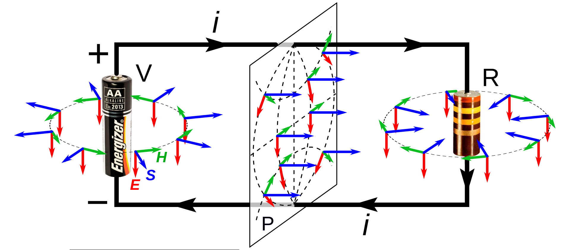
In any case… The next thing I should discuss is field momentum. Indeed, if we’ve got flow, we’ve got momentum. But I’ll leave that for my next post. This topic can’t be exhausted in one post only, indeed. 🙂 So let me conclude this post. I’ll do with a very nice illustration I got from the Wikipedia article on the Poynting vector. It shows the Poynting vector around a voltage source and a resistor, as well as what’s going on in-between. [Note that the magnetic field is given by the field vector H, which is related to B as follows: B = μ₀(H + M), with M the magnetization of the medium. B and H are obviously just proportional in empty space, with μ₀ as the proportionality constant.]

Some content on this page was disabled on June 16, 2020 as a result of a DMCA takedown notice from The California Institute of Technology. You can learn more about the DMCA here:

https://en.support.wordpress.com/copyright-and-the-dmca/
Some content on this page was disabled on June 16, 2020 as a result of a DMCA takedown notice from The California Institute of Technology. You can learn more about the DMCA here:

https://en.support.wordpress.com/copyright-and-the-dmca/
Some content on this page was disabled on June 16, 2020 as a result of a DMCA takedown notice from The California Institute of Technology. You can learn more about the DMCA here:

https://en.support.wordpress.com/copyright-and-the-dmca/
Some content on this page was disabled on June 16, 2020 as a result of a DMCA takedown notice from The California Institute of Technology. You can learn more about the DMCA here:

https://en.support.wordpress.com/copyright-and-the-dmca/
Some content on this page was disabled on June 16, 2020 as a result of a DMCA takedown notice from The California Institute of Technology. You can learn more about the DMCA here:

https://en.support.wordpress.com/copyright-and-the-dmca/
Some content on this page was disabled on June 16, 2020 as a result of a DMCA takedown notice from The California Institute of Technology. You can learn more about the DMCA here:

https://en.support.wordpress.com/copyright-and-the-dmca/
Some content on this page was disabled on June 16, 2020 as a result of a DMCA takedown notice from The California Institute of Technology. You can learn more about the DMCA here:

https://en.support.wordpress.com/copyright-and-the-dmca/
Some content on this page was disabled on June 16, 2020 as a result of a DMCA takedown notice from The California Institute of Technology. You can learn more about the DMCA here:

https://en.support.wordpress.com/copyright-and-the-dmca/
Some content on this page was disabled on June 16, 2020 as a result of a DMCA takedown notice from The California Institute of Technology. You can learn more about the DMCA here:

https://en.support.wordpress.com/copyright-and-the-dmca/
Some content on this page was disabled on June 16, 2020 as a result of a DMCA takedown notice from The California Institute of Technology. You can learn more about the DMCA here:

https://en.support.wordpress.com/copyright-and-the-dmca/
Some content on this page was disabled on June 16, 2020 as a result of a DMCA takedown notice from The California Institute of Technology. You can learn more about the DMCA here:

https://en.support.wordpress.com/copyright-and-the-dmca/
Some content on this page was disabled on June 16, 2020 as a result of a DMCA takedown notice from The California Institute of Technology. You can learn more about the DMCA here:

https://en.support.wordpress.com/copyright-and-the-dmca/
Some content on this page was disabled on June 16, 2020 as a result of a DMCA takedown notice from The California Institute of Technology. You can learn more about the DMCA here:

https://en.support.wordpress.com/copyright-and-the-dmca/
Some content on this page was disabled on June 16, 2020 as a result of a DMCA takedown notice from The California Institute of Technology. You can learn more about the DMCA here:

https://en.support.wordpress.com/copyright-and-the-dmca/
Some content on this page was disabled on June 16, 2020 as a result of a DMCA takedown notice from The California Institute of Technology. You can learn more about the DMCA here:

https://en.support.wordpress.com/copyright-and-the-dmca/
Some content on this page was disabled on June 17, 2020 as a result of a DMCA takedown notice from Michael A. Gottlieb, Rudolf Pfeiffer, and The California Institute of Technology. You can learn more about the DMCA here:

https://en.support.wordpress.com/copyright-and-the-dmca/
Some content on this page was disabled on June 20, 2020 as a result of a DMCA takedown notice from Michael A. Gottlieb, Rudolf Pfeiffer, and The California Institute of Technology. You can learn more about the DMCA here:

https://en.support.wordpress.com/copyright-and-the-dmca/