Fields and charges (II)

Pre-script (dated 26 June 2020): This post has become less relevant (even irrelevant, perhaps) because my views on all things quantum-mechanical have evolved significantly as a result of my progression towards a more complete realist (classical) interpretation of quantum physics. In addition, some of the material was removed by a dark force (that also created problems with the layout, I see now). In any case, we recommend you read our recent papers. I keep blog posts like these mainly because I want to keep track of where I came from. I might review them one day, but I currently don’t have the time or energy for it. 🙂

Original post:

My previous posts was, perhaps, too full of formulas, without offering much reflection. Let me try to correct that here by tying up a few loose ends. The first loose end is about units. Indeed, I haven’t been very clear about that and so let me somewhat more precise on that now.

Note: In case you’re not interested in units, you can skip the first part of this post. However, please do look at the section on the electric constant ε₀ and, most importantly, the section on natural units—especially Planck units, as I will touch upon the topic of gauge coupling parameters there and, hence, on quantum mechanics. Also, the third and last part, on the theoretical contradictions inherent in the idea of point charges, may be of interest to you.]

The field energy integrals

When we wrote that down that u = ε₀E²/2 formula for the energy density of an electric field (see my previous post on fields and charges for more details), we noted that the 1/2 factor was there to avoid double-counting. Indeed, those volume integrals we use to calculate the energy over all space (i.e. U = ∫(u)dV) count the energy that’s associated with a pair of charges (or, to be precise, charge elements) twice and, hence, they have a 1/2 factor in front. Indeed, as Feynman notes, there is no convenient way, unfortunately, of writing an integral that keeps track of the pairs so that each pair is counted just once. In fact, I’ll have to come back to that assumption of there being ‘pairs’ of charges later, as that’s another loose end in the theory.

Now, we also said that that ε₀ factor in the second integral (i.e. the one with the vector dot product E•E =|E||E|cos(0) = E²) is there to make the units come out alright. Now, when I say that, what does it mean really? I’ll explain. Let me first make a few obvious remarks:

1. Densities are always measures in terms per unit volume, so that’s the cubic meter (m³). That’s, obviously, an astronomical unit at the atomic or molecular scale.
2. Because of historical reasons, the conventional unit of charge is not the so-called elementary charge +e (i.e. the charge of a proton), but the coulomb. Hence, the charge density ρ is expressed in Coulomb per cubic meter (C/m³). The coulomb is a rather astronomical unit too—at the atomic or molecular scale at least: 1 e ≈ 1.6022×10⁻¹⁹ C. [I am rounding here to four digits after the decimal point.]
3. Energy is in joule (J) and that’s, once again, a rather astronomical unit at the lower end of the scales. Indeed, theoretical physicists prefer to use the electronvolt (eV), which is the energy gained (or lost) when an electron (so that’s a charge of –e, i.e. minus e) moves across a potential difference of one volt. But so we’ll stick to the joule as for now, not the eV, because the joule is the SI unit that’s used when defining most electrical units, such as the ampere, the watt and… Yes. The volt. Let’s start with that one.

The volt

The volt unit (V) measures both potential (energy) as well as potential difference (in both cases, we mean electric potential only, of course). Now, from all that you’ve read so far, it should be obvious that potential (energy) can only be measured with respect to some reference point. In physics, the reference point is infinity, which is so far away from all charges that there is no influence there. Hence, any charge we’d bring there (i.e. at infinity) will just stay where it is and not be attracted or repelled by anything. We say the potential there is zero: Φ(∞) = 0. The choice of that reference point allows us, then, to define positive or negative potential: the potential near positive charges will be positive and, vice versa, the potential near negative charges will be negative. Likewise, the potential difference between the positive and negative terminal of a battery will be positive.

So you should just note that we measure both potential as well as potential difference in volt and, hence, let’s now answer the question of what a volt really is. The answer is quite straightforward: the potential at some point r = (x, y, z) measures the work done when bringing one unit charge (i.e. +e) from infinity to that point. Hence, it’s only natural that we define one volt as one joule per unit charge:

1 volt = 1 joule/coulomb (1 V = 1 J/C).

Also note the following:

1. One joule is the energy energy transferred (or work done) when applying a force of one newton over a distance of one meter, so one volt can also be measured in newton·meter per coulomb: 1 V = 1 J/C = N·m/C.
2. One joule can also be written as 1 J = 1 V·C.

It’s quite easy to see why that energy = volt-coulomb product makes sense: higher voltage will be associated with higher energy, and the same goes for higher charge. Indeed, the so-called ‘static’ on our body is usually associated with potential differences of thousands of volts (I am not kidding), but the charges involved are extremely small, because the ability of our body to store electric charge is minimal (i.e. the capacitance (aka capacity) of our body). Hence, the shock involved in the discharge is usually quite small: it is measured in milli-joules (mJ), indeed.

The farad

The remark on ‘static’ brings me to another unit which I should mention in passing: the farad. It measures the capacitance (formerly known as the capacity) of a capacitor (formerly known as a condenser). A condenser consists, quite simply, of two separated conductors: it’s usually illustrated as consisting of two plates or of thin foils (e.g. aluminum foil) separated by an insulating film (e.g. waxed paper), but one can also discuss the capacity of a single body, like our human body, or a charged sphere. In both cases, however, the idea is the same: we have a ‘positive’ charge on one side (+q), and a ‘negative’ charge on the other (–q). In case of a single object, we imagine the ‘other’ charge to be some other large object (the Earth, for instance, but it can also be a car or whatever object that could potentially absorb the charge on our body) or, in case of the charged sphere, we could imagine some other sphere of much larger radius. The farad will then measure the capacity of one or both conductors to store charge.

Now, you may think we don’t need another unit here if that’s the definition: we could just express the capacity of a condensor in terms of its maximum ‘load’, couldn’t we? So that’s so many coulomb before the thing breaks down, when the waxed paper fails to separate the two opposite charges on the aluminium foil, for example. No. It’s not like that. It’s true we can not continue to increase the charge without consequences. However, what we want to measure with the farad is another relationship. Because of the opposite charges on both sides, there will be a potential difference, i.e. a voltage difference. Indeed, a capacitor is like a little battery in many ways: it will have two terminals. Now, it is fairly easy to show that the potential difference (i.e. the voltage) between the two plates will be proportional to the charge. Think of it as follows: if we double the charges, we’re doubling the fields, right? So then we need to do twice the amount of work to carry the unit charge (against the field) from one plate to the other. Now, because the distance is the same, that means the potential difference must be twice what it was.

Now, while we have a simple proportionality here between the voltage and the charge, the coefficient of proportionality will depend on the type of conductors, their shape, the distance and the type of insulator (aka dielectric) between them, and so on and so on. Now, what’s being measured in farad is that coefficient of proportionality, which we’ll denote by C_Q (the proportionality coefficient for the charge), C_V ((the proportionality coefficient for the voltage) or, because we should make a choice between the two, quite simply, as C. Indeed, we can either write (1) Q = C_QV or, alternatively, V = C_VQ, with C_Q = 1/C_V. As Feynman notes, “someone originally wrote the equation of proportionality as Q = CV”, so that’s what it will be: the capacitance (aka capacity) of a capacitor (aka condenser) is the ratio of the electric charge Q (on each conductor) to the potential difference V between the two conductors. So we know that’s a constant typical of the type of condenser we’re talking about. Indeed, the capacitance is the constant of proportionality defining the linear relationship between the charge and the voltage means doubling the voltage, and so we can write:

C = Q/V

Now, the charge is measured in coulomb, and the voltage is measured in volt, so the unit in which we will measure C is coulomb per volt (C/V), which is also known as the farad (F):

1 farad = 1 coulomb/volt (1 F = 1 C/V)

[Note the confusing use of the same symbol C for both the unit of charge (coulomb) as well as for the proportionality coefficient! I am sorrry about that, but so that’s convention!].

To be precise, I should add that the proportionality is generally there, but there are exceptions. More specifically, the way the charge builds up (and the way the field builds up, at the edges of the capacitor, for instance) may cause the capacitance to vary a little bit as it is being charged (or discharged). In that case, capacitance will be defined in terms of incremental changes: C = dQ/dV.

Let me conclude this section by giving you two formulas, which are also easily proved but so I will just give you the result:

1. The capacity of a parallel-plate condenser is C = ε₀A/d. In this formula, we have, once again, that ubiquitous electric constant ε₀ (think of it as just another coefficient of proportionality), and then A, i.e. the area of the plates, and d, i.e. the separation between the two plates.
2. The capacity of a charged sphere of radius r (so we’re talking the capacity of a single conductor here) is C = 4πε₀r. This may remind you of the formula for the surface of a sphere (A = 4πr²), but note we’re not squaring the radius. It’s just a linear relationship with r.

I am not giving you these two formulas to show off or fill the pages, but because they’re so ubiquitous and you’ll need them. In fact, I’ll need the second formula in this post when talking about the other ‘loose end’ that I want to discuss.

Other electrical units

From your high school physics classes, you know the ampere and the watt, of course:

1. The ampere is the unit of current, so it measures the quantity of charge moving or circulating per second. Hence, one ampere is one coulomb per second: 1 A = 1 C/s.
2. The watt measures power. Power is the rate of energy conversion or transfer with respect to time. One watt is one joule per second: 1 W = 1 J/s = 1 N·m/s. Also note that we can write power as the product of current and voltage: 1 W = (1 A)·(1 V) = (1 C/s)·(1 J/C) = 1 J/s.

Now, because electromagnetism is such well-developed theory and, more importantly, because it has so many engineering and household applications, there are many other units out there, such as:

• The ohm (Ω): that’s the unit of electrical resistance. Let me quickly define it: the ohm is defined as the resistance between two points of a conductor when a (constant) potential difference (V) of one volt, applied to these points, produces a current (I) of one ampere. So resistance (R) is another proportionality coefficient: R = V/I, and 1 ohm (Ω) = 1 volt/ampere (V/A). [Again, note the (potential) confusion caused by the use of the same symbol (V) for voltage (i.e. the difference in potential) as well as its unit (volt).] Now, note that it’s often useful to write the relationship as V = R·I, so that gives the potential difference as the product of the resistance and the current.
• The weber (Wb) and the tesla (T): that’s the unit of magnetic flux (i.e. the strength of the magnetic field) and magnetic flux density (i.e. one tesla = one weber per square meter) respectively. So these have to do with the field vector B, rather than E. So we won’t talk about it here.
• The henry (H): that’s the unit of electromagnetic inductance. It’s also linked to the magnetic effect. Indeed, from Maxwell’s equations, we know that a changing electric current will cause the magnetic field to change. Now, a changing magnetic field causes circulation of E. Hence, we can make the unit charge go around in some loop (we’re talking circulation of E indeed, not flux). The related energy, or the work that’s done by a unit of charge as it travels (once) around that loop, is – quite confusingly! – referred to as electromotive force (emf). [The term is quite confusing because we’re not talking force but energy, i.e. work, and, as you know by now, energy is force times distance, so energy and force are related but not the same.] To ensure you know what we’re talking about, let me note that emf is measured in volts, so that’s in joule per coulomb: 1 V = 1 J/C. Back to the henry now. If the rate of change of current in a circuit (e.g. the armature winding of an electric motor) is one ampere per second, and the resulting electromotive force (remember: emf is energy per coulomb) is one volt, then the inductance of the circuit is one henry. Hence, 1 H = 1 V/(1 A/s) = 1 V·s/A.     

The concept of impedance

You’ve probably heard about the so-called impedance of a circuit. That’s a complex concept, literally, because it’s a complex-valued ratio. I should refer you to the Web for more details, but let me try to summarize it because, while it’s complex, that doesn’t mean it’s complicated. 🙂 In fact, I think it’s rather easy to grasp after all you’ve gone through already. 🙂 So let’s give it a try.

When we have a simple direct current (DC), then we have a very straightforward definition of resistance (R), as mentioned above: it’s a simple ratio between the voltage (as measured in volt) and the current (as measured in ampere). Now, with alternating current (AC) circuits, it becomes more complicated, and so then it’s the concept of impedance that kicks in. Just like resistance, impedance also sort of measures the ‘opposition’ that a circuit presents to a current when a voltage is applied, but we have a complex ratio—literally: it’s a ratio with a magnitude and a direction, or a phase as it’s usually referred to. Hence, one will often write the impedance (denoted by Z) using Euler’s formula:

Z = |Z|e^iθ

Now, if you don’t know anything about complex numbers, you should just skip all of what follows and go straight to the next section. However, if you do know what a complex number is (it’s an ‘arrow’, basically, and if θ is a variable, then it’s a rotating arrow, or a ‘stopwatch hand’, as Feynman calls it in his more popular Lectures on QED), then you may want to carry on reading.

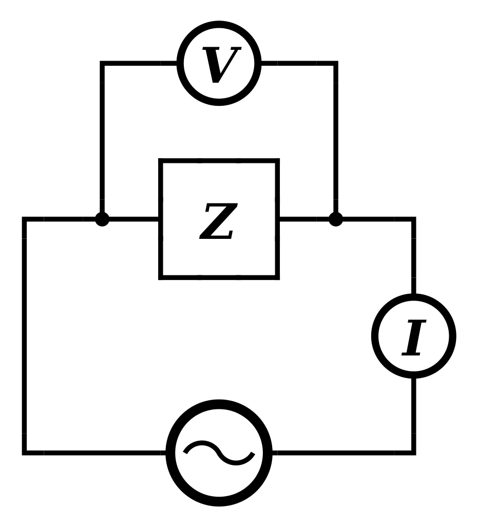
The illustration below (credit goes to Wikipedia, once again) is, probably, the most generic view of an AC circuit that one can jot down. If we apply an alternating current, both the current as well as the voltage will go up and down. However, the current signal will lag the voltage signal, and the phase factor θ tells us by how much. Hence, using complex-number notation, we write:

V = I∗Z = I∗|Z|e^iθ

Now, while that resembles the V = R·I formula I mentioned when discussing resistance, you should note the bold-face type for V and I, and the ∗ symbol I am using here for multiplication. First the ∗ symbol: that’s a convention Feynman adopts in the above-mentioned popular account of quantum mechanics. I like it, because it makes it very clear we’re not talking a vector cross product A×B here, but a product of two complex numbers. Now, that’s also why I write V and I in bold-face: they have a phase too and, hence, we can write them as:

• V = |V|e^{i(ωt + θ_V)}
• I = |I|e^{i(ωt + θ_I)}

This works out as follows:

V = I∗Z = |I|e^{i(ωt + θ_I)}∗|Z|e^iθ = |I||Z|e^{i(ωt + θ_I + θ)} = |V|e^{i(ωt + θ_V)}

Indeed, because the equation must hold for all t, we can equate the magnitudes and phases and, hence, we get: |V| = |I||Z| and θ_V = θ_I + θ. But voltage and current is something real, isn’t it? Not some complex number? You’re right. The complex notation is used mainly to simplify the calculus, but it’s only the real part of those complex-valued functions that count. [In any case, because we limit ourselves to complex exponentials here, the imaginary part (which is the sine, as opposed to the real part, which is the cosine) is the same as the real part, but with a lag of its own (π/2 or 90 degrees, to be precise). Indeed: when writing Euler’s formula out (e^iθ = cos(θ) + isin(θ), you should always remember that the sine and cosine function are basically the same function: they differ only in the phase, as is evident from the trigonometric identity sin(θ+π/) = cos(θ).]

Now, that should be more than enough in terms of an introduction to the units used in electromagnetic theory. Hence, let’s move on.

The electric constant ε₀

Let’s now look at  that energy density formula once again. When looking at that u = ε₀E²/2 formula, you may think that its unit should be the square of the unit in which we measure field strength. How do we measure field strength? It’s defined as the force on a unit charge (E = F/q), so it should be newton per coulomb (N/C). Because the coulomb can also be expressed in newton·meter/volt (1 V = 1 J/C = N·m/C and, hence, 1 C = 1 N·m/V), we can express field strength not only in newton/coulomb but also in volt per meter: 1 N/C = 1 N·V/N·m = 1 V/m. How do we get from N²/C² and/or V²/m² to J/m³?

Well… Let me first note there’s no issue in terms of units with that ρΦ formula in the first integral for U: [ρ]·[Φ] = (C/m³)·V = [(N·m/V)/m³)·V = (N·m)/m³ = J/m³. No problem whatsoever. It’s only that second expression for U, with the u = ε₀E²/2 in the integrand, that triggers the question. Here, we just need to accept that we need that ε₀ factor to make the units come out alright. Indeed, just like other physical constants (such as c, G, or h, for example), it has a dimension: its unit is either C²/N·m² or, what amounts to the same, C/V·m. So the units come out alright indeed if, and only if, we multiply the N²/C² and/or V²/m² units with the dimension of ε₀:

1. (N²/C²)·(C²/N·m²) = (N²·m)·(1/m³) = J/m³
2. (V²/m²)·(C/V·m) = V·C/m³ = (V·N·m/V)/m³ = N·m/m³ = J/m³

Done! 

But so that’s the units only. The electric constant also has a numerical value:

ε₀ = 8.854187817…×10⁻¹² C/V·m ≈ 8.8542×10⁻¹² C/V·m

This numerical value of ε₀ is as important as its unit to ensure both expressions for U yield the same result. Indeed, as you may or may not remember from the second of my two posts on vector calculus, if we have a curl-free field C (that means ∇×C = 0 everywhere, which is the case when talking electrostatics only, as we are doing here), then we can always find some scalar field ψ such that C = ∇ψ. But so here we have E = –ε₀∇Φ, and so it’s not the minus sign that distinguishes the expression from the C = ∇ψ expression, but the ε₀ factor in front.

It’s just like the vector equation for heat flow: h = –κ∇T. Indeed, we also have a constant of proportionality here, which is referred to as the thermal conductivity. Likewise, the electric constant ε₀ is also referred to as the permittivity of the vacuum (or of free space), for similar reasons obviously!

Natural units

You may wonder whether we can’t find some better units, so we don’t need the rather horrendous 8.8542×10⁻¹² C/V·m factor (I am rounding to four digits after the decimal point). The answer is: yes, it’s possible. In fact, there are several systems in which the electric constant (and the magnetic constant, which we’ll introduce later) reduce to 1. The best-known are the so-called Gaussian and Lorentz-Heaviside units respectively.

Gauss defined the unit of charge in what is now referred to as the statcoulomb (statC), which is also referred to as the franklin (Fr) and/or the electrostatic unit of charge (esu), but I’ll refer you to the Wikipedia article on it in case you’d want to find out more about it. You should just note the definition of this unit is problematic in other ways. Indeed, it’s not so easy to try to define ‘natural units’ in physics, because there are quite a few ‘fundamental’ relations and/or laws in physics and, hence, equating this or that constant to one usually has implications on other constants. In addition, one should note that many choices that made sense as ‘natural’ units in the 19th century seem to be arbitrary now. For example:

1. Why would we select the charge of the electron or the proton as the unit charge (+1 or –1) if we now assume that protons (and neutrons) consists of quarks, which have +2/3 or –1/3?
2. What unit would we choose as the unit for mass, knowing that, despite all of the simplification that took place as a result of the generalized acceptance of the quark model, we’re still stuck with quite a few elementary particles whose mass would be a ‘candidate’ for the unit mass? Do we chose the electron, the u quark, or the d quark?

Therefore, the approach to ‘natural units’ has not been to redefine mass or charge or temperature, but the physical constants themselves. Obvious candidates are, of course, c and ħ, i.e. the speed of light and Planck’s constant. [You may wonder why physicists would select ħ, rather than h, as a ‘natural’ unit, but I’ll let you think about that. The answer is not so difficult.] That can be done without too much difficulty indeed, and so one can equate some more physical constants with one. The next candidate is the so-called Boltzmann constant (k_B). While this constant is not so well known, it does pop up in a great many equations, including those that led Planck to propose his quantum of action, i.e. h (see my post on Planck’s constant). When we do that – so when we equate c, ħ and k_B with one (c = ħ = k_B = 1), we still have a great many choices, so we need to impose further constraints. The next is to equate the gravitational constant with one, so then we have c = ħ = k_B = G = 1.

Now, it turns out that the ‘solution’ of this ‘set’ of four equations (c = ħ = k_B = G = 1) does, effectively, lead to ‘new’ values for most of our SI base units, most notably length, time, mass and temperature. These ‘new’ units are referred to as Planck units. You can look up their values yourself, and I’ll let you appreciate the ‘naturalness’ of the new units yourself. They are rather weird. The Planck length and time are usually referred to as the smallest possible measurable units of length and time and, hence, they are related to the so-called limits of quantum theory. Likewise, the Planck temperature is a related limit in quantum theory: it’s the largest possible measurable unit of temperature. To be frank, it’s hard to imagine what the scale of the Planck length, time and temperature really means. In contrast, the scale of the Planck mass is something we actually can imagine – it is said to correspond to the mass of an eyebrow hair, or a flea egg – but, again, its physical significance is not so obvious: Nature’s maximum allowed mass for point-like particles, or the mass capable of holding a single elementary charge. That triggers the question: do point-like charges really exist? I’ll come back to that question. But first I’ll conclude this little digression on units by introducing the so-called fine-structure constant, of which you’ve surely heard before.

The fine-structure constant

I wrote that the ‘set’ of equations c = ħ = k_B = G = 1 gave us Planck units for most of our SI base units. It turns out that these four equations do not lead to a ‘natural’ unit for electric charge. We need to equate a fifth constant with one to get that. That fifth constant is Coulomb’s constant (often denoted as k_e) and, yes, it’s the constant that appears in Coulomb’s Law indeed, as well as in some other pretty fundamental equations in electromagnetics, such as the field caused by a point charge q: E = q/4πε₀r². Hence, k_e = 1/4πε₀. So if we equate k_e with one, then ε₀ will, obviously, be equal to ε₀ = 1/4π.

To make a long story short, adding this fifth equation to our set of five also gives us a Planck charge, and I’ll give you its value: it’s about 1.8755×10⁻¹⁸ C. As I mentioned that the elementary charge is 1 e ≈ 1.6022×10⁻¹⁹ C, it’s easy to that the Planck charge corresponds to some 11.7 times the charge of the proton. In fact, let’s be somewhat more precise and round, once again, to four digits after the decimal point: the q_P/e ratio is about 11.7062. Conversely, we can also say that the elementary charge as expressed in Planck units, is about 1/11.7062 ≈ 0.08542455. In fact, we’ll use that ratio in a moment in some other calculation, so please jot it down.

0.08542455? That’s a bit of a weird number, isn’t it? You’re right. And trying to write it in terms of the charge of a u or d quark doesn’t make it any better. Also, note that the first four significant digits (8542) correspond to the first four significant digits after the decimal point of our ε₀ constant. So what’s the physical significance here? Some other limit of quantum theory?

Frankly, I did not find anything on that, but the obvious thing to do is to relate is to what is referred to as the fine-structure constant, which is denoted by α. This physical constant is dimensionless, and can be defined in various ways, but all of them are some kind of ratio of a bunch of these physical constants we’ve been talking about:

The only constants you have not seen before are μ₀, R_K and, perhaps, r_e as well as m_e . However, these can be defined as a function of the constants that you did see before:

1. The μ₀ constant is the so-called magnetic constant. It’s something similar as ε₀ and it’s referred to as the magnetic permeability of the vacuum. So it’s just like the (electric) permittivity of the vacuum (i.e. the electric constant ε₀) and the only reason why you haven’t heard of this before is because we haven’t discussed magnetic fields so far. In any case, you know that the electric and magnetic force are part and parcel of the same phenomenon (i.e. the electromagnetic interaction between charged particles) and, hence, they are closely related. To be precise, μ₀ = 1/ε₀c². That shows the first and second expression for α are, effectively, fully equivalent.
2. Now, from the definition of k_e = 1/4πε₀, it’s easy to see how those two expressions are, in turn, equivalent with the third expression for α.
3. The R_K constant is the so-called von Klitzing constant, but don’t worry about it: it’s, quite simply, equal to R_K = h/e². Hene, substituting (and don’t forget that h = 2πħ) will demonstrate the equivalence of the fourth expression for α.
4. Finally, the r_e factor is the classical electron radius, which is usually written as a function of m_e, i.e. the electron mass: r_e = e²/4πε₀m_ec². This very same equation implies that r_em_e = e²/4πε₀c². So… Yes. It’s all the same really.

Let’s calculate its (rounded) value in the old units first, using the third expression:

• The e² constant is (roughly) equal to (1.6022×10^–19 C)² = 2.5670×10^–38 C². Coulomb’s constant k_e = 1/4πε₀ is about 8.9876×10⁹ N·m²/C². Hence, the numerator e²k_e ≈ 23.0715×10^–29 N·m².
• The (rounded) denominator is ħc = (1.05457×10^–34 N·m·s)(2.998×10⁸ m/s) = 3.162×10^–26 N·m².
• Hence, we get α = k_ee²/ħc ≈ 7.297×10^–3 = 0.007297.

Note that this number is, effectively, dimensionless. Now, the interesting thing is that if we calculate α using Planck units, we get an e² constant that is (roughly) equal to 0.08542455² = … 0.007297! Now, because all of the other constants are equal to 1 in Planck’s system of units, that’s equal to α itself. So… Yes ! The two values for α are one and the same in the two systems of units and, of course, as you might have guessed, the fine-structure constant is effectively dimensionless because it does not depend on our units of measurement. So what does it correspond to?

Now that would take me a very long time to explain, but let me try to summarize what it’s all about. In my post on quantum electrodynamics (QED) – so that’s the theory of light and matter basically and, most importantly, how they interact – I wrote about the three basic events in that theory, and how they are associated with a probability amplitude, so that’s a complex number, or an ‘arrow’, as Feynman puts it: something with (a) a magnitude and (b) a direction. We had to take the absolute square of these amplitudes in order to calculate the probability (i.e. some real number between 0 and 1) of the event actually happening. These three basic events or actions were:

1. A photon travels from point A to B. To keep things simple and stupid, Feynman denoted this amplitude by P(A to B), and please note that the P stands for photon, not for probability. I should also note that we have an easy formula for P(A to B): it depends on the so-called space-time interval between the two points A and B, i.e. I = Δr² – Δt² = (x₂–x₁)²+(y₂–y₁)²+(z₂–z₁)² – (t₂–t₁)². Hence, the space-time interval takes both the distance in space as well as the ‘distance’ in time into account.
2. An electron travels from point A to B: this was denoted by E(A to B) because… Well… You guessed it: the E of electron. The formula for E(A to B) was much more complicated, but the two key elements in the formula was some complex number j (see below), and some other (real) number n.
3. Finally, an electron could emit or absorb a photon, and the amplitude associated with this event was denoted by j, for junction.

Now, that junction number j is about –0.1. To be somewhat more precise, I should say it’s about –0.08542455.

–0.08542455? That’s a bit of a weird number, isn’t it? Hey ! Didn’t we see this number somewhere else? We did, but before you scroll up, let’s first interpret this number. It looks like an ordinary (real) number, but it’s an amplitude alright, so you should interpret it as an arrow. Hence, it can be ‘combined’ (i.e. ‘added’ or ‘multiplied’) with other arrows. More in particular, when you multiply it with another arrow, it amounts to a shrink to a bit less than one-tenth (because its magnitude is about 0.085 = 8.5%), and half a turn (the minus sign amounts to a rotation of 180°). Now, in that post of mine, I wrote that I wouldn’t entertain you on the difficulties of calculating this number but… Well… We did see this number before indeed. Just scroll up to check it. We’ve got a very remarkable result here:

j ≈ –0.08542455 = –√0.007297 = –√α = –e expressed in Planck units

So we find that our junction number j or – as it’s better known – our coupling constant in quantum electrodynamics (aka as the gauge coupling parameter g) is equal to the (negative) square root of that fine-structure constant which, in turn, is equal to the charge of the electron expressed in the Planck unit for electric charge. Now that is a very deep and fundamental result which no one seems to be able to ‘explain’—in an ‘intuitive’ way, that is.

I should immediately add that, while we can’t explain it, intuitively, it does make sense. A lot of sense actually. Photons carry the electromagnetic force, and the electromagnetic field is caused by stationary and moving electric charges, so one would expect to find some relation between that junction number j, describing the amplitude to emit or absorb a photon, and the electric charge itself, but… An equality? Really?

Well… Yes. That’s what it is, and I look forward to trying to understand all of this better. For now, however, I should proceed with what I set out to do, and that is to tie up a few loose ends. This was one, and so let’s move to the next, which is about the assumption of point charges.

Note: More popular accounts of quantum theory say α itself is ‘the’ coupling constant, rather than its (negative) square –√α = j = –e (expressed in Planck units). That’s correct: g or j are, technically speaking, the (gauge) coupling parameter, not the coupling constant. But that’s a little technical detail which shouldn’t bother you. The result is still what it is: very remarkable! I should also note that it’s often the value of the reciprocal (1/α) that is specified, i.e. 1/0.007297 ≈ 137.036. But so now you know what this number actually stands for. 🙂

Do point charges exist?

Feynman’s Lectures on electrostatics are interesting, among other things, because, besides highlighting the precision and successes of the theory, he also doesn’t hesitate to point out the contradictions. He notes, for example, that “the idea of locating energy in the field is inconsistent with the assumption of the existence of point charges.”

Huh?

Yes. Let’s explore the point. We do assume point charges in classical physics indeed. The electric field caused by a point charge is, quite simply:

E = q/4πε₀r²

Hence, the energy density u is ε₀E²/2 = q²/32πε₀r⁴. Now, we have that volume integral U = (ε₀/2)∫E•EdV = ∫(ε₀E²/2)dV integral. As Feynman notes, nothing prevents us from taking a spherical shell for the volume element dV, instead of an infinitesimal cube. This spherical shell would have the charge q at its center, an inner radius equal to r, an infinitesimal thickness dr, and, finally, a surface area 4πr² (that’s just the general formula for the surface area of a spherical shell, which I also noted above). Hence, its (infinitesimally small) volume is 4πr²dr, and our integral becomes:

To calculate this integral, we need to take the limit of –q²/8πε₀r for (a) r tending to zero (r→0) and for (b) r tending to infinity (r→∞). The limit for r = ∞ is zero. That’s OK and consistent with the choice of our reference point for calculating the potential of a field. However, the limit for r = 0 is zero is infinity! Hence, that U = (ε₀/2)∫E•EdV basically says there’s an infinite amount of energy in the field of a point charge! How is that possible? It cannot be true, obviously.

So… Where did we do wrong?

Your first reaction may well be that this very particular approach (i.e. replacing our infinitesimal cubes by infinitesimal shells) to calculating our integral is fishy and, hence, not allowed. Maybe you’re right. Maybe not. It’s interesting to note that we run into similar problems when calculating the energy of a charged sphere. Indeed, we mentioned the formula for the capacity of a charged sphere: C = 4πε₀r. Now, there’s a similarly easy formula for the energy of a charged sphere. Let’s look at how we charge a condenser:

• We know that the potential difference between two plates of a condenser represents the work we have to do, per unit charge, to transfer a charge (Q) from one plate to the other. Hence, we can write V = ΔU/ΔQ.
• We will, of course, want to do a differential analysis. Hence, we’ll transfer charges incrementally, one infinitesimal little charge dQ at the time, and re-write V as V = dU/dQ or, what amounts to the same: dU = V·dQ.
• Now, we’ve defined the capacitance of a condenser as C = Q/V. [Again, don’t be confused: C stands for capacity here, measured in coulomb per volt, not for the coulomb unit.] Hence, we can re-write dU as dU = Q·dQ/C.
• Now we have to integrate dU going from zero charge to the final charge Q. Just do a little bit of effort here and try it. You should get the following result: U = Q²/2C. [We could re-write this as U = (C²/V²)/2C =  C·V²/2, which is a form that may be more useful in some other context but not here.]
• Using that C = 4πε₀r formula, we get our grand result. The energy of a charged sphere is:

U = Q²/8πε₀r

From that formula, it’s obvious that, if the radius of our sphere goes to zero, its energy should also go to infinity! So it seems we can’t really pack a finite charge Q in one single point. Indeed, to do that, our formula says we need an infinite amount of energy. So what’s going on here?

Nothing much. You should, first of all, remember how we got that integral: see my previous post for the full derivation indeed. It’s not that difficult. We first assumed we had pairs of charges q_i and q_j for which we calculated the total electrostatic energy U as the sum of the energies of all possible pairs of charges:

And, then, we looked at a continuous distribution of charge. However, in essence, we still did the same: we counted the energy of interaction between infinitesimal charges situated at two different points (referred to as point 1 and 2 respectively), with a 1/2 factor in front so as to ensure we didn’t double-count (there’s no way to write an integral that keeps track of the pairs so that each pair is counted only once):

Now, we reduced this double integral by a clever substitution to something that looked a bit better:

Finally, some more mathematical tricks gave us that U = (ε₀/2)∫E•EdV integral.

In essence, what’s wrong in that integral above is that it actually includes the energy that’s needed to assemble the finite point charge q itself from an infinite number of infinitesimal parts. Now that energy is infinitely large. We just can’t do it: the energy required to construct a point charge is ∞.

Now that explains the physical significance of that Planck mass ! We said Nature has some kind of maximum allowable mass for point-like particles, or the mass capable of holding a single elementary charge. What’s going on is, as we try to pile more charge on top of the charge that’s already there, we add energy. Now, energy has an equivalent mass. Indeed, the Planck charge (q_P ≈ 1.8755×10⁻¹⁸ C), the Planck length (l_P = 1.616×10⁻³⁵ m), the Planck energy (1.956×10⁹ J), and the Planck mass (2.1765×10⁻⁸ kg) are all related. Now things start making sense. Indeed, we said that the Planck mass is tiny but, still, it’s something we can imagine, like a flea’s egg or the mass of a hair of a eyebrow. The associated energy (E = mc², so that’s (2.1765×10⁻⁸ kg)·(2.998×10⁸ m/s)² ≈ 19.56×10⁸ kg·m²/s² = 1.956×10⁹ joule indeed.

Now, how much energy is that? Well… That’s about 2 giga-joule, obviously, but so what’s that in daily life? It’s about the energy you would get when burning 40 liter of fuel. It’s also likely to amount, more or less, to your home electricity consumption over a month. So it’s sizable, and so we’re packing all that energy into a Planck volume (l_P³ ≈ 4×10⁻¹⁰⁵ m³). If we’d manage that, we’d be able to create tiny black holes, because that’s what that little Planck volume would become if we’d pack so much energy in it. So… Well… Here I just have to refer you to more learned writers than I am. As Wikipedia notes dryly: “The physical significance of the Planck length is a topic of theoretical research. Since the Planck length is so many orders of magnitude smaller than any current instrument could possibly measure, there is no way of examining it directly.”

So… Well… That’s it for now. The point to note is that we would not have any theoretical problems if we’d assume our ‘point charge’ is actually not a point charge but some small distribution of charge itself. You’ll say: Great! Problem solved! 

Well… For now, yes. But Feynman rightly notes that assuming that our elementary charges do take up some space results in other difficulties of explanation. As we know, these difficulties are solved in quantum mechanics, but so we’re not supposed to know that when doing these classical analyses. 🙂

Some content on this page was disabled on June 17, 2020 as a result of a DMCA takedown notice from Michael A. Gottlieb, Rudolf Pfeiffer, and The California Institute of Technology. You can learn more about the DMCA here:

https://en.support.wordpress.com/copyright-and-the-dmca/