
Pre-script (dated 26 June 2020): This post has become less relevant (even irrelevant, perhaps) because my views on all things quantum-mechanical have evolved significantly as a result of my progression towards a more complete realist (classical) interpretation of quantum physics. In addition, some of the material was removed by a dark force (that also created problems with the layout, I see now). In any case, we recommend you read our recent papers. I keep blog posts like these mainly because I want to keep track of where I came from. I might review them one day, but I currently don’t have the time or energy for it. 🙂
Original post:
My previous posts focused mainly on photons, so this one should be focused more on matter-particles, things that have a mass and a charge. However, I will use it more as an opportunity to talk about fields and present some results from electrostatics using our new vector differential operators (see my posts on vector analysis).
Before I do so, let me note something that is obvious but… Well… Think about it: photons carry the electromagnetic force, but have no electric charge themselves. Likewise, electromagnetic fields have energy and are caused by charges, but so they also carry no charge. So… Fields act on a charge, and photons interact with electrons, but it’s only matter-particles (notably the electron and the proton, which is made of quarks) that actually carry electric charge. Does that make sense? It should. 🙂
Another thing I want to remind you of, before jumping into it all head first, are the basic units and relations that are valid always, regardless of what we are talking about. They are represented below:
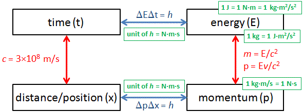
Let me recapitulate the main points:
- The speed of light is always the same, regardless of the reference frame (inertial or moving), and nothing can travel faster than light (except mathematical points, such as the phase velocity of a wavefunction).
- This universal rule is the basis of relativity theory and the mass-energy equivalence relation E = mc2.
- The constant speed of light also allows us to redefine the units of time and/or distance such that c = 1. For example, if we re-define the unit of distance as the distance traveled by light in one second, or the unit of time as the time light needs to travel one meter, then c = 1.
- Newton’s laws of motion define a force as the product of a mass and its acceleration: F = m·a. Hence, mass is a measure of inertia, and the unit of force is 1 newton (N) = 1 kg·m/s2.
- The momentum of an object is the product of its mass and its velocity: p = m·v. Hence, its unit is 1 kg·m/s = 1 N·s. Therefore, the concept of momentum combines force (N) as well as time (s).
- Energy is defined in terms of work: 1 Joule (J) is the work done when applying a force of one newton over a distance of one meter: 1 J = 1 N·m. Hence, the concept of energy combines force (N) and distance (m).
- Relativity theory establishes the relativistic energy-momentum relation pc = Ev/c, which can also be written as E2 = p2c2 + m02c4, with m0 the rest mass of an object (i.e. its mass when the object would be at rest, relative to the observer, of course). These equations reduce to m = E and E2 = p2 + m02 when choosing time and/or distance units such that c = 1. The mass m is the total mass of the object, including its inertial mass as well as the equivalent mass of its kinetic energy.
- The relationships above establish (a) energy and time and (b) momentum and position as complementary variables and, hence, the Uncertainty Principle can be expressed in terms of both. The Uncertainty Principle, as well as the Planck-Einstein relation and the de Broglie relation (not shown on the diagram), establish a quantum of action, h, whose dimension combines force, distance and time (h ≈ 6.626×10⁻³⁴ N·m·s). This quantum of action (Wirkung) can be defined in various ways, as it pops up in more than one fundamental relation, but one of the more obvious approaches is to define h as the proportionality constant between the energy of a photon (i.e. the ‘light particle’) and its frequency: h = E/ν.
Note that we talked about forces and energy above, but we didn’t say anything about the origin of these forces. That’s what we are going to do now, even if we’ll limit ourselves to the electromagnetic force only.
Electrostatics
According to Wikipedia, electrostatics deals with the phenomena and properties of stationary or slow-moving electric charges with no acceleration. Feynman usually uses the term when talking about stationary charges only. If a current is involved (i.e. slow-moving charges with no acceleration), the term magnetostatics is preferred. However, the distinction does not matter all that much because – remarkably! – with stationary charges and steady currents, the electric and magnetic fields (E and B) can be analyzed as separate fields: there is no interconnection whatsoever! That shows, mathematically, as a neat separation between (1) Maxwell’s first and second equation and (2) Maxwell’s third and fourth equation:
- Electrostatics: (i) ∇•E = ρ/ε0 and (ii) ∇×E = 0.
- Magnetostatics: (iii) c2∇×B = j/ε0 and (iv) ∇•B = 0.
Electrostatics: The ρ in equation (i) is the so-called charge density, which describes the distribution of electric charges in space: ρ = ρ(x, y, z). To put it simply: ρ is the ‘amount of charge’ (which we’ll denote by Δq) per unit volume at a given point. As for ε0, that’s a constant which ensures all units are ‘compatible’. Equation (i) basically says we have some flux of E, the exact amount of which is determined by the charge density ρ or, more in general, by the charge distribution in space. As for equation (ii), i.e. ∇×E = 0, we can sort of forget about that. It means the curl of E is zero: everywhere, and always. So there’s no circulation of E. Hence, E is a so-called curl-free field, in this case at least, i.e. when only stationary charges and steady currents are involved.
Magnetostatics: The j in (iii) represents a steady current indeed, causing some circulation of B. The c2 factor is related to the fact that magnetism is actually only a relativistic effect of electricity, but I can’t dwell on that here. I’ll just refer you to what Feynman writes about this in his Lectures, and warmly recommend to read it. Oh… Equation (iv), ∇•B = 0, means that the divergence of B is zero: everywhere, and always. So there’s no flux of B. None. So B is a divergence-free field.
Because of the neat separation, we’ll just forget about B and talk about E only.
The electric potential
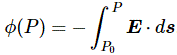
OK. Let’s try to go through the motions as quickly as we can. As mentioned in my introduction, energy is defined in terms of work done. So we should just multiply the force and the distance, right? 1 Joule = 1 newton × 1 meter, right? Well… Yes and no. In discussions like this, we talk potential energy, i.e. energy stored in the system, so to say. That means that we’re looking at work done against the force, like when we carry a bucket of water up to the third floor or, to use a somewhat more scientific description of what’s going on, when we are separating two masses. Because we’re doing work against the force, we put a minus sign in front of our integral:

Now, the electromagnetic force works pretty much like gravity, except that, when discussing gravity, we only have positive ‘charges’ (the mass of some object is always positive). In electromagnetics, we have positive as well as negative charge, and please note that two like charges repel (that’s not the case with gravity). Hence, doing work against the electromagnetic force may involve bringing like charges together or, alternatively, separating opposite charges. We can’t say. Fortunately, when it comes to the math of it, it doesn’t matter: we will have the same minus sign in front of our integral. The point is: we’re doing work against the force, and so that’s what the minus sign stands for. So it has nothing to do with the specifics of the law of attraction and repulsion in this case (electromagnetism as opposed to gravity) and/or the fact that electrons carry negative charge. No.
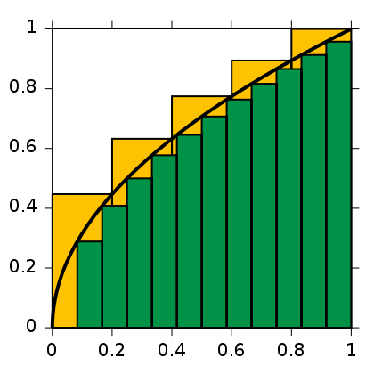
Let’s get back to the integral. Just in case you forgot, the integral sign ∫ stands for an S: the S of summa, i.e. sum in Latin, and we’re using these integrals because we’re adding an infinite number of infinitesimally small contributions to the total effort here indeed. You should recognize it, because it’s a general formula for energy or work. It is, once again, a so-called line integral, so it’s a bit different than the ∫f(x)dx stuff you learned from high school. Not very different, but different nevertheless. What’s different is that we have a vector dot product F•ds after the integral sign here, so that’s not like f(x)dx. In case you forgot, that f(x)dx product represents the surface of an infinitesimally rectangle, as shown below: we make the base of the rectangle smaller and smaller, so dx becomes an infinitesimal indeed. And then we add them all up and get the area under the curve. If f(x) is negative, then the contributions will be negative.
But so we don’t have little rectangles here. We have two vectors, F and ds, and their vector dot product, F•ds, which will give you… Well… I am tempted to write: the tangential component of the force along the path, but that’s not quite correct: if ds was a unit vector, it would be true—because then it’s just like that h•n product I introduced in our first vector calculus class. However, ds is not a unit vector: it’s an infinitesimal vector, and, hence, if we write the tangential component of the force along the path as Ft, then F•ds = |F||ds|cosθ = F·cosθ·ds = Ft·ds. So this F•ds is a tangential component over an infinitesimally small segment of the curve. In short, it’s an infinitesimally small contribution to the total amount of work done indeed. You can make sense of this by looking at the geometrical representation of the situation below.
I am just saying this so you know what that integral stands for. Note that we’re not adding arrows once again, like we did when calculating amplitudes or so. It’s all much more straightforward really: a vector dot product is a scalar, so it’s just some real number—just like any component of a vector (tangential, normal, in the direction of one of the coordinates axes, or in whatever direction) is not a vector but a real number. Hence, W is also just some real number. It can be positive or negative because… Well… When we’d be going down the stairs with our bucket of water, our minus sign doesn’t disappear. Indeed, our convention to put that minus sign there should obviously not depend on what point a and b we’re talking about, so we may actually be going along the direction of the force when going from a to b.
As a matter of fact, you should note that’s actually the situation which is depicted above. So then we get a negative number for W. Does that make sense? Of course it does: we’re obviously not doing any work here as we’re moving along the direction, so we’re surely not adding any (potential) energy to the system. On the contrary, we’re taking energy out of the system. Hence, we are reducing its (potential) energy and, hence, we should have a negative value for W indeed. So, just think of the minus sign being there to ensure we add potential energy to the system when going against the force, and reducing it when going with the force.
OK. You get this. You probably also know we’ll re-define W as a difference in potential between two points, which we’ll write as Φ(b) – Φ(a). Now that should remind you of your high school integral ∫f(x)dx once again. For a definite integral over a line segment [a, b], you’d have to find the antiderivative of f(x), which you’d write as F(x), and then you’d take the difference F(b) – F(a) too. Now, you may or may not remember that this antiderivative was actually a family of functions F(x) + k, and k could be any constant – 5/9, 6π, 3.6×10124, 0.86, whatever! – because such constant vanishes when taking the derivative.
Here we have the same, we can define an infinite number of functions Φ(r) + k, of which the gradient will yield… Stop! I am going too fast here. First, we need to re-write that W function above in order to ensure we’re calculating stuff in terms of the unit charge, so we write:
Huh? Well… Yes. I am using the definition of the field E here really: E is the force (F) when putting a unit charge in the field. Hence, if we want the work done per unit charge, i.e. W(unit), then we have to integrate the vector dot product E·ds over the path from a to b. But so now you see what I want to do. It makes the comparison with our high school integral complete. Instead of taking a derivative in regard to one variable only, i.e. dF(x)/dx) = f(x), we have a function Φ here not in one but in three variables: Φ = Φ(x, y, z) = Φ(r) and, therefore, we have to take the vector derivative (or gradient as it’s called) of Φ to get E:
∇Φ(x, y, z) = (∂Φ/∂x, ∂Φ/∂y, ∂Φ/∂z) = –E(x, y, z)
But so it’s the same principle as what you learned how to use to solve your high school integral. Now, you’ll usually see the expression above written as:
E = –∇Φ
Why so short? Well… We all just love these mysterious abbreviations, don’t we? 🙂 Jokes aside, it’s true some of those vector equations pack an awful lot of information. Just take Feynman’s advice here: “If it helps to write out the components to be sure you understand what’s going on, just do it. There is nothing inelegant about that. In fact, there is often a certain cleverness in doing just that.” So… Let’s move on.
I should mention that we can only apply this more sophisticated version of the ‘high school trick’ because Φ and E are like temperature (T) and heat flow (h): they are fields. T is a scalar field and h is a vector field, and so that’s why we can and should apply our new trick: if we have the scalar field, we can derive the vector field. In case you want more details, I’ll just refer you to our first vector calculus class. Indeed, our so-called First Theorem in vector calculus was just about the more sophisticated version of the ‘high school trick’: if we have some scalar field ψ (like temperature or potential, for example: just substitute the ψ in the equation below for T or Φ), then we’ll always find that:
The Γ here is the curve between point 1 and 2, so that’s the path along which we’re going, and ∇ψ must represent some vector field.
Let’s go back to our W integral. I should mention that it doesn’t matter what path we take: we’ll always get the same value for W, regardless of what path we take. That’s why the illustration above showed two possible paths: it doesn’t matter which one we take. Again, that’s only because E is a vector field. To be precise, the electrostatic field is a so-called conservative vector field, which means that we can’t get energy out of the field by first carrying some charge along one path, and then carrying it back along another. You’ll probably find that’s obvious, and it is. Just note it somewhere in the back of your mind.
So we’re done. We should just substitute E for ∇Φ, shouldn’t we? Well… Yes. For minus ∇Φ, that is. Another minus sign. Why? Well… It makes that W(unit) integral come out alright. Indeed, we want a formula like W = Φ(b) – Φ(a), not like Φ(a) – Φ(b). Look at it. We could, indeed, define E as the (positive) gradient of some scalar field ψ = –Φ, and so we could write E = ∇ψ, but then we’d find that W = –[ψ(b) – ψ(a)] = ψ(a) – ψ(b).
You’ll say: so what? Well… Nothing much. It’s just that our field vectors would point from lower to higher values of ψ, so they would be flowing uphill, so to say. Now, we don’t want that in physics. Why? It just doesn’t look good. We want our field vectors to be directed from higher potential to lower potential, always. Just think of it: heat (h) flows from higher temperature (T) to lower, and Newton’s apple falls from greater to lower height. Likewise, when putting a unit charge in the field, we want to see it move from higher to lower electric potential. Now, we can’t change the direction of E, because that’s the direction of the force and Nature doesn’t care about our conventions and so we can’t choose the direction of the force. But we can choose our convention. So that’s why we put a minus sign in front of ∇Φ when writing E = –∇Φ. It makes everything come out alright. 🙂 That’s why we also have a minus sign in the differential heat flow equation: h = –κ∇T.
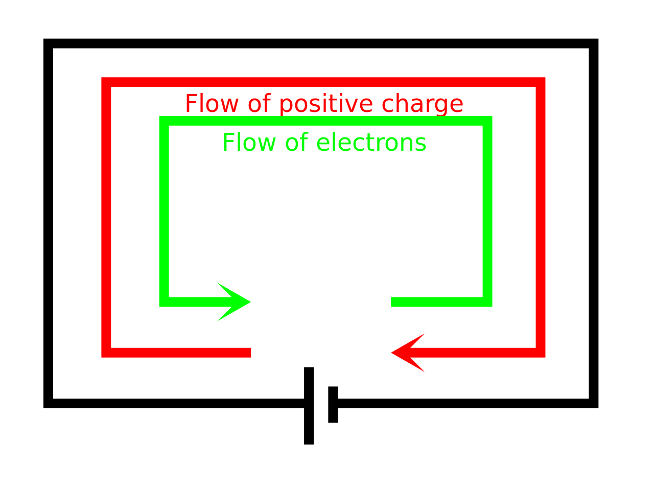
So now we have the easy W(unit) = Φ(b) – Φ(a) formula that we wanted all along. Now, note that, when we say a unit charge, we mean a plus one charge. Yes: +1. So that’s the charge of the proton (it’s denoted by e) so you should stop thinking about moving electrons around! [I am saying this because I used to confuse myself by doing that. You end up with the same formulas for W and Φ but it just takes you longer to get there, so let me save you some time here. :-)]
But… Yes? In reality, it’s electrons going through a wire, isn’t? Not protons. Yes. But it doesn’t matter. Units are units in physics, and they’re always +1, for whatever (time, distance, charge, mass, spin, etcetera). Always. For whatever. Also note that in laboratory experiments, or particle accelerators, we often use protons instead of electrons, so there’s nothing weird about it. Finally, and most fundamentally, if we have a –e charge moving through a neutral wire in one direction, then that’s exactly the same as a +e charge moving in the other way.
Just to make sure you get the point, let’s look at that illustration once again. We already said that we have F and, hence, E pointing from a to b and we’ll be reducing the potential energy of the system when moving our unit charge from a to b, so W was some negative value. Now, taking into account we want field lines to point from higher to lower potential, Φ(a) should be larger than Φ(b), and so… Well.. Yes. It all makes sense: we have a negative difference Φ(b) – Φ(a) = W(unit), which amounts, of course, to the reduction in potential energy.
The last thing we need to take care of now, is the reference point. Indeed, any Φ(r) + k function will do, so which one do we take? The approach here is to take a reference point P0 at infinity. What’s infinity? Well… Hard to say. It’s a place that’s very far away from all of the charges we’ve got lying around here. Very far away indeed. So far away we can say there is nothing there really. No charges whatsoever. 🙂 Something like that. 🙂 In any case. I need to move on. So Φ(P0) is zero and so we can finally jot down the grand result for the electric potential Φ(P) (aka as the electrostatic or electric field potential):
So now we can calculate all potentials, i.e. when we know where the charges are at least. I’ve shown an example below. As you can see, besides having zero potential at infinity, we will usually also have one or more equipotential surfaces with zero potential. One could say these zero potential lines sort of ‘separate’ the positive and negative space. That’s not a very scientifically accurate description but you know what I mean.
Let me make a few final notes about the units. First, let me, once again, note that our unit charge is plus one, and it will flow from positive to negative potential indeed, as shown below, even if we know that, in an actual electric circuit, and so now I am talking about a copper wire or something similar, that means the (free) electrons will move in the other direction.
 If you’re smart (and you are), you’ll say: what about the right-hand rule for the magnetic force? Well… We’re not discussing the magnetic force here but, because you insist, rest assured it comes out alright. Look at the illustration below of the magnetic force on a wire with a current, which is a pretty standard one.
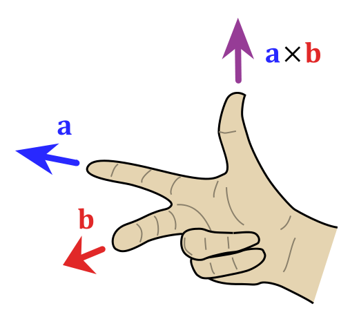
So we have a given B, because of the bar magnet, and then v, the velocity vector for the… Electrons? No. You need to be consistent. It’s the velocity vector for the unit charges, which are positive (+e). Now just calculate the force F = qv×B = ev×B using the right-hand rule for the vector cross product, as illustrated below. So v is the thumb and B is the index finger in this case. All you need to do is tilt your hand, and it comes out alright.
But… We know it’s electrons going the other way. Well… If you insist. But then you have to put a minus sign in front of the q, because we’re talking minus e (–e). So now v is in the other direction and so v×B is in the other direction indeed, but our force F = qv×B = –ev×B is not. Fortunately not, because physical reality should not depend on our conventions. 🙂 So… What’s the conclusion. Nothing. You may or may not want to remember that, when we say that our current j current flows in this or that direction, we actually might be talking electrons (with charge minus one) flowing in the opposite direction, but then it doesn’t matter. In addition, as mentioned above, in laboratory experiments or accelerators, we may actually be talking protons instead of electrons, so don’t assume electromagnetism is the business of electrons only.
To conclude this disproportionately long introduction (we’re finally ready to talk more difficult stuff), I should just make a note on the units. Electric potential is measured in volts, as you know. However, it’s obvious from all that I wrote above that it’s the difference in potential that matters really. From the definition above, it should be measured in the same unit as our unit for energy, or for work, so that’s the joule. To be precise, it should be measured in joule per unit charge. But here we have one of the very few inconsistencies in physics when it comes to units. The proton is said to be the unit charge (e), but its actual value is measured in coulomb (C). To be precise: +1 e = 1.602176565(35)×10−19 C. So we do not measure voltage – sorry, potential difference 🙂 – in joule but in joule per coulomb (J/C).
Now, we usually use another term for the joule/coulomb unit. You guessed it (because I said it): it’s the volt (V). One volt is one joule/coulomb: 1 V = 1 J/C. That’s not fair, you’ll say. You’re right, but so the proton charge e is not a so-called SI unit. Is the Coulomb an SI unit? Yes. It’s derived from the ampere (A) which, believe it or not, is actually an SI base unit. One ampere is 6.241×10¹⁸ electrons (i.e. one coulomb) per second. You may wonder how the ampere (or the coulomb) can be a base unit. Can they be expressed in terms of kilogram, meter and second, like all other base units. The answer is yes but, as you can imagine, it’s a bit of a complex description and so I’ll refer you to the Web for that.
The Poisson equation
I started this post by saying that I’d talk about fields and present some results from electrostatics using our ‘new’ vector differential operators, so it’s about time I do that. The first equation is a simple one. Using our E = –∇Φ formula, we can re-write the ∇•E = ρ/ε0 equation as:
∇•E = ∇•∇Φ = ∇2Φ = –ρ/ε0
This is a so-called Poisson equation. The ∇2 operator is referred to as the Laplacian and is sometimes also written as Δ, but I don’t like that because it’s also the symbol for the total differential, and that’s definitely not the same thing. The formula for the Laplacian is given below. Note that it acts on a scalar field (i.e. the potential function Φ in this case).
![]() As Feynman notes: “The entire subject of electrostatics is merely the study of the solutions of this one equation.” However, I should note that this doesn’t prevent Feynman from devoting at least a dozen of his Lectures on it, and they’re not the easiest ones to read. [In case you’d doubt this statement, just have a look at his lecture on electric dipoles, for example.] In short: don’t think the ‘study of this one equation’ is easy. All I’ll do is just note some of the most fundamental results of this ‘study’.
As Feynman notes: “The entire subject of electrostatics is merely the study of the solutions of this one equation.” However, I should note that this doesn’t prevent Feynman from devoting at least a dozen of his Lectures on it, and they’re not the easiest ones to read. [In case you’d doubt this statement, just have a look at his lecture on electric dipoles, for example.] In short: don’t think the ‘study of this one equation’ is easy. All I’ll do is just note some of the most fundamental results of this ‘study’.
Also note that ∇•E is one of our ‘new’ vector differential operators indeed: it’s the vector dot product of our del operator (∇) with E. That’s something very different than, let’s say, ∇Φ. A little dot and some bold-face type make an enormous difference here. 🙂 You may or may remember that we referred to the ∇• operator as the divergence (div) operator (see my post on that).
Gauss’ Law
Gauss’ Law is not to be confused with Gauss’ Theorem, about which I wrote elsewhere. It gives the flux of E through a closed surface S, any closed surface S really, as the sum of all charges inside the surface divided by the electric constant ε0 (but then you know that constant is just there to make the units come out alright).
The derivation of Gauss’ Law is a bit lengthy, which is why I won’t reproduce it here, but you should note its derivation is based, mainly, on the fact that (a) surface areas are proportional to r2 (so if we double the distance from the source, the surface area will quadruple), and (b) the magnitude of E is given by an inverse-square law, so it decreases as 1/r2. That explains why, if the surface S describes a sphere, the number we get from Gauss’ Law is independent of the radius of the sphere. The diagram below (credit goes to Wikipedia) illustrates the idea.
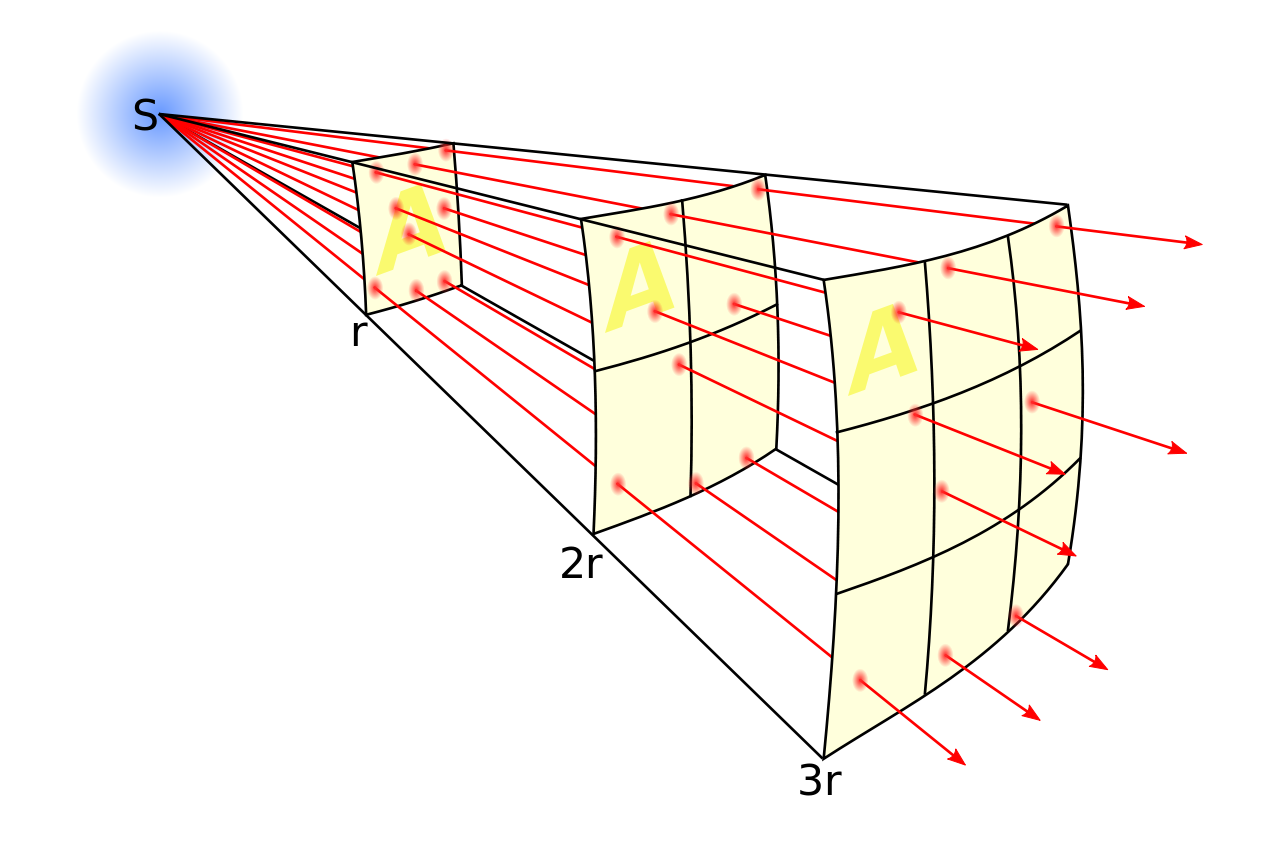
The diagram can be used to show how a field and its flux can be represented. Indeed, the lines represent the flux of E emanating from a charge. Now, the total number of flux lines depends on the charge but is constant with increasing distance because the force is radial and spherically symmetric. A greater density of flux lines (lines per unit area) means a stronger field, with the density of flux lines (i.e. the magnitude of E) following an inverse-square law indeed, because the surface area of a sphere increases with the square of the radius. Hence, in Gauss’ Law, the two effect cancel out: the two factors vary with distance, but their product is a constant.
Now, if we describe the location of charges in terms of charge densities (ρ), then we can write Qint as:
Now, Gauss’ Law also applies to an infinitesimal cubical surface and, in one of my posts on vector calculus, I showed that the flux of E out of such cube is given by ∇•E·dV. At this point, it’s probably a good idea to remind you of what this ‘new’ vector differential operator ∇•, i.e. our ‘divergence’ operator, stands for: the divergence of E (i.e. ∇• applied to E, so that’s ∇•E) represents the volume density of the flux of E out of an infinitesimal volume around a given point. Hence, it’s the flux per unit volume, as opposed to the flux out of the infinitesimal cube itself, which is the product of ∇•E and dV, i.e. ∇•E·dV.
So what? Well… Gauss’ Law applied to our infinitesimal volume gives us the following equality:
![]()
That, in turn, simplifies to:
![]()
So that’s Maxwell’s first equation once again, which is equivalent to our Poisson equation: ∇•E = ∇2Φ = –ρ/ε0. So what are we doing here? Just listing equivalent formulas? Yes. I should also note they can be derived from Coulomb’s law of force, which is probably the one you learned in high school. So… Yes. It’s all consistent. But then that’s what we should expect, of course. 🙂
The energy in a field
All these formulas look very abstract. It’s about time we use them for something. A lot of what’s written in Feynman’s Lectures on electrostatics is applied stuff indeed: it focuses, among other things, on calculating the potential in various circumstances and for various distributions of charge. Now, funnily enough, while that ∇•E = –ρ/ε0 equation is equivalent to Coulomb’s law and, obviously, much more compact to write down, Coulomb’s law is easier to start with for basic calculations. Let me first write Coulomb’s law. You’ll probably recognize it from your high school days:
F1 is the force on charge q1, and F2 is the force on charge q2. Now, q1 and q2. may attract or repel each other but, in both cases, the forces will be equal and opposite. [In case you wonder, yes, that’s basically the law of action and reaction.] The e12 vector is the unit vector from q2 to q1, not from q1 to q2, as one might expect. That’s because we’re not talking gravity here: like charges do not attract but repel and, hence, we have to switch the order here. Having said that, that’s basically the only peculiar thing about the equation. All the rest is standard:
- The force is inversely proportional to the square of the distance and so we have an inverse-square law here indeed.
- The force is proportional to the charge(s).
- Finally, we have a proportionality constant, 1/4πε0, which makes the units come out alright. You may wonder why it’s written the way it’s written, i.e. with that 4π factor, but that factor (4π or 2π) actually disappears in a number of calculations, so then we will be left with just a 1/ε0 or a 1/2ε0 factor. So don’t worry about it.
We want to calculate potentials and all that, so the first thing we’ll do is calculate the force on a unit charge. So we’ll divide that equation by q1, to calculate E(1) = F1/q1:
Piece of cake. But… What’s E(1) really? Well… It’s the force on the unit charge (+e), but so it doesn’t matter whether or not that unit charge is actually there, so it’s the field E caused by a charge q2. [If that doesn’t make sense to you, think again.] So we can drop the subscripts and just write:
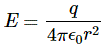
What a relief, isn’t it? The simplest formula ever: the (magnitude) of the field as a simple function of the charge q and its distance (r) from the point that we’re looking at, which we’ll write as P = (x, y, z). But what origin are we using to measure x, y and z. Don’t be surprised: the origin is q.
Now that’s a formula we can use in the Φ(P) integral. Indeed, the antiderivative is ∫(q/4πε0r2)dr. Now, we can bring q/4πε0 out and so we’re left with ∫(1/r2)dr. Now ∫(1/r2)dr is equal to –1/r + k, and so the whole antiderivative is –q/4πε0r + k. However, the minus sign cancels out with the minus sign in front of the Φ(P) = Φ(x, y, z) integral, and so we get:
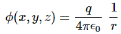
You should just do the integral to check this result. It’s the same integral but with P0 (infinity) as point a and P as point b in the integral, so we have ∞ as start value and r as end value. The integral then yields Φ(P) – Φ(P0) = –q/4πε0[1/r – 1/∞). [The k constant falls away when subtracting Φ(P0) from Φ(P).] But 1/∞ = 0, and we had a minus sign in front of the integral, which cancels the sign of –q/4πε0. So, yes, we get the wonderfully simple result above. Also please do quickly check if it makes sense in terms of sign: the unit charge is +e, so that’s a positive charge. Hence, Φ(x, y, z) will be positive if the sign of q is also positive, but negative if q would happen to be negative. So that’s OK.
Also note that the potential – which, remember, represents the amount of work to be done when bringing a unit charge (e) from infinity to some distance r from a charge q – is proportional to the charge of q. We also know that the force and, hence, the work is proportional to the charge that we are bringing in (that’s how we calculated the work per unit in the first place: by dividing the total amount of work by the charge). Hence, if we’d not bring some unit charge but some other charge q2, the work done would also be proportional to q2. Now, we need to make sure we understand what we’re writing and so let’s tidy up and re-label our first charge once again as q1, and the distance r as r12, because that’s what r is: the distance between the two charges. We then have another obvious but nice result: the work done in bringing two charges together from a large distance (infinity) is
![]() Now, one of the many nice properties of fields (scalar or vector fields) and the associated energies (because that’s what we are talking about here) is that we can simply add up contributions. For example, if we’d have many charges and we’d want to calculate the potential Φ at a point which we call 1, we can use the same Φ(r) = q/4πε0r formula which we had derived for one charge only, for all charges, and then we simply add the contributions of each to get the total potential:
Now, one of the many nice properties of fields (scalar or vector fields) and the associated energies (because that’s what we are talking about here) is that we can simply add up contributions. For example, if we’d have many charges and we’d want to calculate the potential Φ at a point which we call 1, we can use the same Φ(r) = q/4πε0r formula which we had derived for one charge only, for all charges, and then we simply add the contributions of each to get the total potential:
Now that we’re here, I should, of course, also give the continuum version of this formula, i.e. the formula used when we’re talking charge densities rather than individual charges. The sum then becomes an infinite sum (i.e. an integral), and qj (note that j goes from 2 to n) becomes a variable which we write as ρ(2). We get:
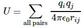
Going back to the discrete situation, we get the same type of sum when bringing multiple pairs of charges qi and qj together. Hence, the total electrostatic energy U is the sum of the energies of all possible pairs of charges:
 It’s been a while since you’ve seen any diagram or so, so let me insert one just to reassure you it’s as simple as that indeed:
Now, we have to be aware of the risk of double-counting, of course. We should not be adding qiqj/4πε0rij twice. That’s why we write ‘all pairs’ under the ∑ summation sign, instead of the usual i, j subscripts. The continuum version of this equation below makes that 1/2 factor explicit:
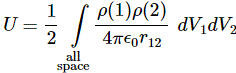
Hmm… What kind of integral is that? It’s a so-called double integral because we have two variables here. Not easy. However, there’s a lucky break. We can use the continuum version of our formula for Φ(1) to get rid of the ρ(2) and dV2 variables and reduce the whole thing to a more standard ‘single’ integral. Indeed, we can write:
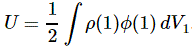 Now, because our point (2) no longer appears, we can actually write that more elegantly as:
 That looks nice, doesn’t it? But do we understand it? Just to make sure. Let me explain it. The potential energy of the charge ρdV is the product of this charge and the potential at the same point. The total energy is therefore the integral over ϕρdV, but then we are counting energies twice, so that’s why we need the 1/2 factor. Now, we can write this even more beautifully as:
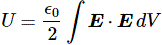
Isn’t this wonderful? We have an expression for the energy of a field, not in terms of the charges or the charge distribution, but in terms of the field they produce.
I am pretty sure that, by now, you must be suffering from ‘formula overload’, so you probably are just gazing at this without even bothering to try to understand. Too bad, and you should take a break then or just go do something else, like biking or so. 🙂
First, you should note that you know this E•E expression already: E•E is just the square of the magnitude of the field vector E, so E•E = E2. That makes sense because we know, from what we know about waves, that the energy is always proportional to the square of an amplitude, and so we’re just writing the same here but with a little proportionality constant (ε0).
OK, you’ll say. But you probably still wonder what use this formula could possibly have. What is that number we get from some integration over all space? So we associate the Universe with some number U and then what? Well… Isn’t that just nice? 🙂 Jokes aside, we’re actually looking at that E•E = E2 product inside of the integral as representing an energy density (i.e. the energy per unit volume). We’ll denote that with a lower-case u symbol and so we write:
![]()
Just to make sure you ‘get’ what we’re talking about here: u is the energy density in the little cube dV in the rather simplistic (and, therefore, extremely useful) illustration below (which, just like most of what I write above, I got from Feynman).
Now that should make sense to you—I hope. 🙂 In any case, if you’re still with me, and if you’re not all formula-ed out you may wonder how we get that ε0E•E = ε0E2 expression from that ρΦ expression. Of course, you know that E = –∇Φ, and we also have the Poisson equation ∇2Φ = –ρ/ε0, but that doesn’t get you very far. It’s one of those examples where an easy-looking formula requires a lot of gymnastics. However, as the objective of this post is to do some of that, let me take you through the derivation.
Let’s do something with that Poisson equation first, so we’ll re-write it as ρ = –ε0∇2Φ, and then we can substitute ρ in the integral with the ρΦ product. So we get:
Now, you should check out those fancy formulas with our new vector differential operators which we listed in our second class on vector calculus, but, unfortunately, none of them apply. So we have to write it all out and see what we get:
Now that looks horrendous and so you’ll surely think we won’t get anywhere with that. Well… Physicists don’t despair as easily as we do, it seems, and so they do substitute it in the integral which, of course, becomes an even more monstrous expression, because we now have two volume integrals instead of one! Indeed, we get:
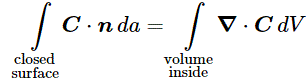
![]() But if ∇Φ is a vector field (it’s minus E, remember!), then Φ∇Φ is a vector field too, and we can then apply Gauss’ Theorem, which we mentioned in our first class on vector calculus, and which – mind you! – has nothing to do with Gauss’ Law. Indeed, Gauss produced so much it’s difficult to keep track of it all. 🙂 So let me remind you of this theorem. [I should also show why Φ∇Φ still yields a field, but I’ll assume you believe me.] Gauss’ Theorem basically shows how we can go from a volume integral to a surface integral:
But if ∇Φ is a vector field (it’s minus E, remember!), then Φ∇Φ is a vector field too, and we can then apply Gauss’ Theorem, which we mentioned in our first class on vector calculus, and which – mind you! – has nothing to do with Gauss’ Law. Indeed, Gauss produced so much it’s difficult to keep track of it all. 🙂 So let me remind you of this theorem. [I should also show why Φ∇Φ still yields a field, but I’ll assume you believe me.] Gauss’ Theorem basically shows how we can go from a volume integral to a surface integral:
 If we apply this to the second integral in our U expression, we get:
So what? Where are we going with this? Relax. Be patient. What volume and surface are we talking about here? To make sure we have all charges and influences, we should integrate over all space and, hence, the surface goes to infinity. So we’re talking a (spherical) surface of enormous radius R whose center is the origin of our coordinate system. I know that sounds ridiculous but, from a math point of view, it is just the same like bringing a charge in from infinity, which is what we did to calculate the potential. So if we don’t difficulty with infinite line integrals, we should not have difficulty with infinite surface and infinite volumes. That’s all I can, so… Well… Let’s do it.
Let’s look at that product Φ∇Φ•n in the surface integral. Φ is a scalar and ∇Φ is a vector, and so… Well… ∇Φ•n is a scalar too: it’s the normal component of ∇Φ = –E. [Just to make sure, you should note that the way we define the normal unit vector n is such that ∇Φ•n is some positive number indeed! So n will point in the same direction, more or less, as ∇Φ = –E. So the θ angle between ∇Φ = –E and n is surely less than ± 90° and, hence, the cosine factor in the ∇Φ•n = |∇Φ||n|cosθ = |∇Φ|cosθ is positive, and so the whole vector dot product is positive.]
So, we have a product of two scalars here. What happens with them if R goes to infinity? Well… The potential varies as 1/r as we’re going to infinity. That’s obvious from that Φ = (q/4πε0)(1/r) formula: just think of q as some kind of average now, which works because we assume all charges are located within some finite distance, while we’re going to infinity. What about ∇Φ•n? Well… Again assuming that we’re reasonably far away from the charges, we’re talking the density of flux lines here (i.e. the magnitude of E) which, as shown above, follows an inverse-square law, because the surface area of a sphere increases with the square of the radius. So ∇Φ•n varies not as 1/r but as 1/r2. To make a long story short, the whole product Φ∇Φ•n falls of as 1/r goes to infinity. Now, we shouldn’t forget we’re integrating a surface integral here, with r = R, and so it’s R going to infinity. So that surface integral has to go to zero when we include all space. The volume integral still stands however, so our formula for U now consists of one term only, i.e. the volume integral, and so we now have:
Done !
What’s left?
In electrostatics? Lots. Electric dipoles (like polar molecules), electrolytes, plasma oscillations, ionic crystals, electricity in the atmosphere (like lightning!), dielectrics and polarization (including condensers), ferroelectricity,… As soon as we try to apply our theory to matter, things become hugely complicated. But the theory works. Fortunately! 🙂 I have to refer you to textbooks, though, in case you’d want to know more about it. [I am sure you don’t, but then one never knows.]
What I wanted to do is to give you some feel for those vector and field equations in the electrostatic case. We now need to bring magnetic field back into the picture and, most importantly, move to electrodynamics, in which the electric and magnetic field do not appear as completely separate things. No! In electrodynamics, they are fully interconnected through the time derivatives ∂E/∂t and ∂B/∂t. That shows they’re part and parcel of the same thing really: electromagnetism.
But we’ll try to tackle that in future posts. Goodbye for now!
Some content on this page was disabled on June 16, 2020 as a result of a DMCA takedown notice from The California Institute of Technology. You can learn more about the DMCA here:
https://wordpress.com/support/copyright-and-the-dmca/
Some content on this page was disabled on June 16, 2020 as a result of a DMCA takedown notice from The California Institute of Technology. You can learn more about the DMCA here:https://wordpress.com/support/copyright-and-the-dmca/
Some content on this page was disabled on June 16, 2020 as a result of a DMCA takedown notice from The California Institute of Technology. You can learn more about the DMCA here:https://wordpress.com/support/copyright-and-the-dmca/
Some content on this page was disabled on June 16, 2020 as a result of a DMCA takedown notice from The California Institute of Technology. You can learn more about the DMCA here:https://wordpress.com/support/copyright-and-the-dmca/
Some content on this page was disabled on June 16, 2020 as a result of a DMCA takedown notice from The California Institute of Technology. You can learn more about the DMCA here:https://wordpress.com/support/copyright-and-the-dmca/
Some content on this page was disabled on June 16, 2020 as a result of a DMCA takedown notice from The California Institute of Technology. You can learn more about the DMCA here:https://wordpress.com/support/copyright-and-the-dmca/
Some content on this page was disabled on June 16, 2020 as a result of a DMCA takedown notice from The California Institute of Technology. You can learn more about the DMCA here:https://wordpress.com/support/copyright-and-the-dmca/
Some content on this page was disabled on June 16, 2020 as a result of a DMCA takedown notice from The California Institute of Technology. You can learn more about the DMCA here:https://wordpress.com/support/copyright-and-the-dmca/
Some content on this page was disabled on June 16, 2020 as a result of a DMCA takedown notice from The California Institute of Technology. You can learn more about the DMCA here:https://wordpress.com/support/copyright-and-the-dmca/
Some content on this page was disabled on June 17, 2020 as a result of a DMCA takedown notice from Michael A. Gottlieb, Rudolf Pfeiffer, and The California Institute of Technology. You can learn more about the DMCA here:https://wordpress.com/support/copyright-and-the-dmca/
Some content on this page was disabled on June 17, 2020 as a result of a DMCA takedown notice from Michael A. Gottlieb, Rudolf Pfeiffer, and The California Institute of Technology. You can learn more about the DMCA here:https://wordpress.com/support/copyright-and-the-dmca/
Some content on this page was disabled on June 17, 2020 as a result of a DMCA takedown notice from Michael A. Gottlieb, Rudolf Pfeiffer, and The California Institute of Technology. You can learn more about the DMCA here:https://wordpress.com/support/copyright-and-the-dmca/
Some content on this page was disabled on June 17, 2020 as a result of a DMCA takedown notice from Michael A. Gottlieb, Rudolf Pfeiffer, and The California Institute of Technology. You can learn more about the DMCA here:https://wordpress.com/support/copyright-and-the-dmca/
Some content on this page was disabled on June 17, 2020 as a result of a DMCA takedown notice from Michael A. Gottlieb, Rudolf Pfeiffer, and The California Institute of Technology. You can learn more about the DMCA here:https://wordpress.com/support/copyright-and-the-dmca/
Some content on this page was disabled on June 17, 2020 as a result of a DMCA takedown notice from Michael A. Gottlieb, Rudolf Pfeiffer, and The California Institute of Technology. You can learn more about the DMCA here:https://wordpress.com/support/copyright-and-the-dmca/
Some content on this page was disabled on June 17, 2020 as a result of a DMCA takedown notice from Michael A. Gottlieb, Rudolf Pfeiffer, and The California Institute of Technology. You can learn more about the DMCA here:https://wordpress.com/support/copyright-and-the-dmca/
Some content on this page was disabled on June 17, 2020 as a result of a DMCA takedown notice from Michael A. Gottlieb, Rudolf Pfeiffer, and The California Institute of Technology. You can learn more about the DMCA here:https://wordpress.com/support/copyright-and-the-dmca/
Some content on this page was disabled on June 17, 2020 as a result of a DMCA takedown notice from Michael A. Gottlieb, Rudolf Pfeiffer, and The California Institute of Technology. You can learn more about the DMCA here:https://wordpress.com/support/copyright-and-the-dmca/
Some content on this page was disabled on June 17, 2020 as a result of a DMCA takedown notice from Michael A. Gottlieb, Rudolf Pfeiffer, and The California Institute of Technology. You can learn more about the DMCA here:https://wordpress.com/support/copyright-and-the-dmca/
Some content on this page was disabled on June 17, 2020 as a result of a DMCA takedown notice from Michael A. Gottlieb, Rudolf Pfeiffer, and The California Institute of Technology. You can learn more about the DMCA here:https://wordpress.com/support/copyright-and-the-dmca/
Some content on this page was disabled on June 17, 2020 as a result of a DMCA takedown notice from Michael A. Gottlieb, Rudolf Pfeiffer, and The California Institute of Technology. You can learn more about the DMCA here:https://wordpress.com/support/copyright-and-the-dmca/
Some content on this page was disabled on June 17, 2020 as a result of a DMCA takedown notice from Michael A. Gottlieb, Rudolf Pfeiffer, and The California Institute of Technology. You can learn more about the DMCA here:https://wordpress.com/support/copyright-and-the-dmca/
Some content on this page was disabled on June 20, 2020 as a result of a DMCA takedown notice from Michael A. Gottlieb, Rudolf Pfeiffer, and The California Institute of Technology. You can learn more about the DMCA here:

4 thoughts on “Fields and charges (I)”