Atomic magnets: precession and diamagnetism

This and the next posts will further build on the concepts introduced in my previous post on particle spin. This post in particular will focus on some of the math we’ll need to understand what quantum mechanics is all about. The first topic is about the quantum-mechanical equivalent of the phenomenon of precession. The other topics are… Well… You’ll see… 🙂

The Larmor frequency

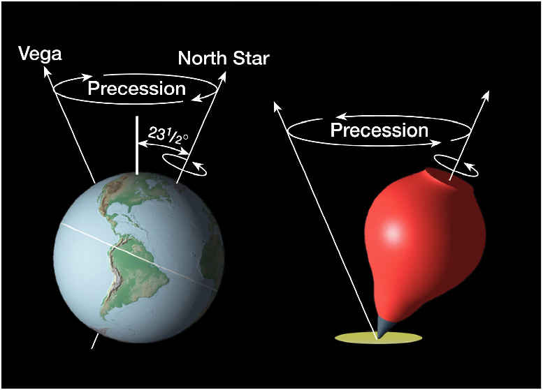
The motion of a spinning object in a force field is quite complicated. In our post on gyroscopes, we introduced the concepts of precession and nutation. The concept of precession is illustrated below for the Earth as well as for a spinning top. In both cases, the external force is just gravity.

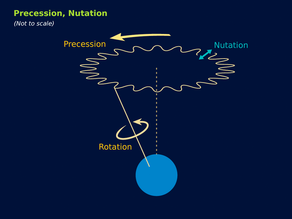
Nutation is an additional movement: on top of the precessional movement, a spinning object may wobble, as illustrated below.

There seems to be no analog for nutation in quantum mechanics. In fact, the terms nutation and precession seem to be used interchangeably in quantum physics, although they are very different in classical physics. But let’s not complicate things and, hence, talk about the phenomenon of precession only.

We will not re-explain the phenomenon of precession here but just remind you that the phenomenon can be described in terms of (a) the angle between the symmetry axis and the momentum vector, which we’ll denote by θ, and (b) the angular velocity of the precession, which we’ll denote by ω_p = dφ/dt, as shown below. The J in the illustration below is the angular momentum of the object. Hence, if we’d imagine it to be an electron, then J would be the spin angular momentum only, not its orbital angular momentum—although the analysis would obviously be valid for the orbital and/or total angular momentum as well.

OK. Let’s look at what’s going on. The angular displacement – which is also, rather confusingly, referred to as the angle of precession – in the time interval Δt is, obviously, equal to Δφ = ω_p·Δt. Now, looking at the geometry of the situation, and using the small-angle approximation for the sine, one can also see that ΔJ ≈ (J·sinθ)·(ω_p·Δt). In fact, going to the limit (i.e. for infinitesimally small Δφ and ΔJ), we can write:

dJ/dt = ω_p·J·sinθ

But the angular momentum cannot change if there’s no torque. In fact, the time rate of change of the angular momentum is equal to the torque. [You should look this up but, if you don’t want to do that, note that this is just the equivalent, for rotational motion, of the F = dp/dt law for linear motion.] Now, in my post on magnetic dipoles, I showed that the torque τ on a loop of current with magnetic moment μ in an external magnetic field B  is equal to τ = μ×B. So the magnitude of the torque is equal to |τ| = |μ|·|B|·sinθ = μ·B·sinθ. Therefore, ω_p·J·sinθ = μ·B·sinθ and, hence,

ω_p = μ·B/J

However, from the general μ/J = –g·(q_e/2m) equation we derived in our previous post, we know that μ/J – for an atomic magnet, that is – must be equal to μ/J = g·q_e/2m. So we get the formula we wanted to get here:

ω_p = g·(q_e/2m)·B

This equation says that the angular velocity of the precession is proportional to the magnitude of the external magnetic field, and that the constant of proportionality is equal to g·(q_e/2m). It’s good to do the math and actually calculate the precession frequency f_p = ω_p/2π. It’s easy. We had calculated q_e/2m already: it was equal to 1.6×10⁻¹⁹ C divided by 2·9.1×10⁻³¹ kg, so that’s 0.0879×10¹²  C/kg or 0.0879×10¹² (C·m)/(N·s²), more or less. 🙂 Now, g is dimensionless, and B is expressed in tesla: 1 T = (N·s)/(C·m), so we get the s⁻¹ dimension we want for a frequency. For g = 2 (so we look at the spin of the electron itself only), we get:

f_p = ω_p/2π = 2·0.0879×10¹²/2π ≈ 28×10⁹ = 28 gigacycles per tesla = 28 GHz/T

This is a number expressed per unit of the magnetic field strength B. Note that you’ll often see this number expressed as 1.4 megacycles per gauss, using the older gauss unit for magnetic field strength: 1 tesla = 10,000 gauss. For a nucleus, we get a somewhat less impressive number because the proton (or neutron) mass is so much bigger: it’s a number expressed in megacycles per tesla, indeed, and for a proton (i.e. a hydrogen nucleus), it’s about 42.58 MHz/T.

Now, you may wonder about the numbers here. Are they astronomical? Maybe. Maybe not. It’s probably good to note that the strength of the magnetic field in medical MRI systems (magnetic resonance imaging systems) is only 1.5 to 3 tesla, so it’s a rather large unit. You should also note that the clock speed of the CPU in your laptop – so that’s the speed at which it executes instructions – is measured in GHz too, so perhaps it’s not so astronomic. I’ll let you judge. 🙂

So… Well… That’s all nice. The key question, of course, is whether or not this classical view of the electron spinning around a proton is accurate, quantum-mechanically, that is. I’ll let Feynman answer that question provisionally:

“According to the classical theory, then, the electron orbits—and spins—in an atom should precess in a magnetic field. Is it also true quantum-mechanically? It is essentially true, but the meaning of the “precession” is different. In quantum mechanics one cannot talk about the direction of the angular momentum in the same sense as one does classically; nevertheless, there is a very close analogy—so close that we continue to call it precession.”

To distinguish classical and quantum-mechanical precession, quantum-mechanical precession is usually referred to as Larmor precession, and the frequencies above are often referred to as Larmor frequencies. However, I should note that, technically speaking, the term Larmor frequency is actually reserved for the frequency I’ll describe in the next section. I should also note that the ω_p = g·(q_e/2m)·B is usually written, quite simply, as ω_p = γ·B. Of course, the gamma is not the Lorentz factor here, but the so-called gyromagnetic ratio (aka as the magnetogyric ratio): γ = g·(q_e/2m). Oh—just so you know: Sir Joseph Larmor was a British physicists and, yes, he developed all of the stuff we’re talking about here. 🙂

At this point, you may wonder if and why all of the above is relevant. Well… There’s more than one answer to this question, but I’d recommend you start with reading the Wikipedia article on NMR spectroscopy. 🙂 And then you should also read Feynman’s exposé on the Rabi atomic or molecular beam method for determining the precession frequency. It’s really fascinating stuff, but you are sufficiently armed now to read those things for yourself, and so I’ll just move on. Indeed, there’s something else I need to talk about here, and that’s Larmor’s Theorem.

Larmor’s Theorem

We’ve been talking single electrons only so far. Now, you may fear that things become quite complicated when many electrons are involved and… Well… That’s true, of course. And then you may also think that things become even more complicated when external fields are involved, like that external magnetic field we introduced above, and that led our electrons to precess at extraordinary frequencies. Well… That’s not true. Here we get some help: Larmor proved a theorem that basically says that, if we can work out the motions of the electrons without the external field, the solution for the motions with the external field is the no-field solution with an added rotation about the axis of the field. More specifically, for an external magnetic field, the added rotation will have an angular frequency equal to:

ω_L = (q_e/2m)·B

So that’s the same formula as we found for the angular velocity of the precession if g = 1, so that’s very easy to remember. The ω_L  frequency, which is the precession frequency for g = 1, is referred to as the Larmor frequency. The proof of the above is remarkably easy, but… Well… I don’t want to copy Feynman here, so I’ll just refer you to the relevant Lecture on it. 🙂

Diamagnetism

I guess it’s about time we relate all of what we learned so far to properties of matter we can relate to, and so that’s what I’ll do here. We’re not going to talk about ferromagnetism here, i.e. the mechanism through which iron, nickel and cobalt and most of their alloys become permanent magnets. That’s quite peculiar and so we will not discuss it here. Here we’ll talk about the very weak quantum-mechanical magnetic effect – a thousand to a million times less than the effects in ferromagnetic materials – that occurs in all materials when placed in an external magnetic field.

While the effect is there in all materials, it’s stronger for some than for others. In fact, it’s usually so weak it is hard to detect, and so it’s usually demonstrated using elements for which the diamagnetic effect is somewhat stronger, like bismuth or antimony. The effect is demonstrated by suspending a piece of material in a non-uniform field, as illustrated below. The diamagnetic effect will cause a small displacement of the material, away from the high-field region, i.e. away from the pointed pole.

I should immediately add that some materials, like aluminium, will actually be attracted to the pointed pole, but that’s because of yet another effect that not all materials share: paramagnetism. I’ll talk about that in another post, together with ferromagnetism. So… Diamagnetism: what is it?

The illustration below shows our spinning electron (q) once again. It also shows a magnetic field B but, unlike our analysis above, or the analysis in our previous post, we assume the external magnetic field is not just there. We assume it changes, because it’s been turned on or off—hopefully slowly: if not, we’d have eddy-current forces causing potentially strong impulses.

But so we’ve got some change in the magnetic flux , and so we know, because of Faraday or Maxwell – you choose 🙂 – that we’ll have some circulation of E, i.e. the electric field. The magnetic flux is B times the surface area, and the circulation is the average tangential component E times the length of the path. Because our model of the orbiting electron is so nice and symmetric, we can write Faraday’s Law here as:

E·2π·r = −d(B·π·r²)/dt ⇔ E = −(r/2)·dB/dt

A field implies a force and, therefore, a torque on the electron. The torque is equal to the force times the lever arm, so it’s equal to (−q_e·E)·r = −q_e·E·r. Of course, the torque is also equal to the rate of the change of the angular momentum, so dJ/dt must equal:

dJ/dt = −q_e·E·r =  q_e·(r/2)·(dB/dt)·r = (q_e·r²/2)·(dB/dt)

Now, the assumption is that the field goes from zero to B, so ΔB = B. Therefore, ΔJ must be equal to:

ΔJ = (q_e·r²/2)·B

You should, in fact, derive this more formally, by integrating—but let’s keep things as simple as we can. 🙂 What does this formula say, really? It’s the extra angular momentum from the ‘twist’ that’s given to the electrons as the field is turned on. Now, this added angular momentum makes an extra magnetic moment which, because it is an orbital motion, is just q_e/2m times the angular momentum that’s already there. But more angular momentum means the magnetic moment has changed, according to the μ = (q_e/2m)·J formula we derived in our previous post, so we have:

Δμ = –(q_e/2m)·ΔJ

The minus sign is there because of Lenz’ law: the added momentum is opposite to the magnetic field—and, yes, I know: it’s hard to keep track of all of the conventions involved here. In any case, we get the following grand equation:

So we found that the induced magnetic moment is directly proportional to the magnetic field B, and opposing it. Now that is what explains why our piece of bismuth does what it does in that non-uniform magnetic field. Of course, you’ll say: why is stronger for bismuth than for other materials? And what about aluminium, or paramagnetism in general? Well… Good questions, but we’ll tackle them in the next posts. 🙂

Let me conclude this post by copying Feynman’s little exposé on why the phenomenon of diamagnetism is so particular. In fact, he notes that, because we’re talking a piece of material here that can’t spin – so it’s held in place, so to say – we should have “no magnetic effects whatsoever”. The reasoning is as follows:

This is very interesting indeed. This classical theorem basically says that the energy of a system should not be affected by the presence of a magnetic field. However, we know magnetic effects, such as the diamagnetic effect, are there, so these effects are referred to as ‘quantum-mechanical’ effects indeed: they cannot be explained using classical theory only, even if all of what we wrote above used classical theory only.

I should also note another point: why do we need a non-homogeneous field? Well… The situation is comparable to what we wrote on the Stern-Gerlach experiment. If we would have a homogeneous magnetic field, then we would only have a torque on all of the atomic magnets, but no net force in one or the other direction. There’s something else here too: you may think that the forces pointing towards and away from the pointed tip should cancel each other out, so there should actually be no net movement of the material at all! Feynman’s analysis works for one atom, indeed, but does it still make sense if we look at the whole piece of material? It does, because we’re talking an induced magnetic moment that’s opposing the field, regardless of the orientation of the magnetic moment of the individual atoms in the piece of material. So, even if the individual atoms have opposite momenta, the extra induced magnetic moment will point in the same direction for all. So that solves that issue. However, it does not address Feynman’s own critical remark in regard to the supposed ‘impossibility’ of diamagnetism in classical mechanics.

But I’ll let you think about this, and sign off for today. 🙂 I hope you enjoyed this post.

Some content on this page was disabled on June 16, 2020 as a result of a DMCA takedown notice from The California Institute of Technology. You can learn more about the DMCA here:

https://en.support.wordpress.com/copyright-and-the-dmca/
Some content on this page was disabled on June 16, 2020 as a result of a DMCA takedown notice from The California Institute of Technology. You can learn more about the DMCA here:

https://en.support.wordpress.com/copyright-and-the-dmca/
Some content on this page was disabled on June 16, 2020 as a result of a DMCA takedown notice from The California Institute of Technology. You can learn more about the DMCA here:

https://en.support.wordpress.com/copyright-and-the-dmca/
Some content on this page was disabled on June 16, 2020 as a result of a DMCA takedown notice from The California Institute of Technology. You can learn more about the DMCA here:

https://en.support.wordpress.com/copyright-and-the-dmca/