Spin

Pre-script (dated 26 June 2020): This post has become less relevant (even irrelevant, perhaps) because my views on all things quantum-mechanical have evolved significantly as a result of my progression towards a more complete realist (classical) interpretation of quantum physics. In addition, some of the material was removed by a dark force (that also created problems with the layout, I see now). In any case, we recommend you read our recent papers. I keep blog posts like these mainly because I want to keep track of where I came from. I might review them one day, but I currently don’t have the time or energy for it. 🙂

Original post:

In the previous posts, I showed how the ‘real-world’ properties of photons and electrons emerge out of very simple mathematical notions and shapes. The basic notions are time and space. The shape is the wavefunction.

Let’s recall the story once again. Space is an infinite number of three-dimensional points (x, y, z), and time is a stopwatch hand going round and round—a cyclical thing. All points in space are connected by an infinite number of paths – straight or crooked, whatever  – of which we measure the length. And then we have ‘photons’ that move from A to B, but so we don’t know what is actually moving in space here. We just associate each and every possible path (in spacetime) between A and B with an amplitude: an ‘arrow‘ whose length and direction depends on (1) the length of the path l (i.e. the ‘distance’ in space measured along the path, be it straight or crooked), and (2) the difference in time between the departure (at point A) and the arrival (at point B) of our photon (i.e. the ‘distance in time’ as measured by that stopwatch hand).

Now, in quantum theory, anything is possible and, hence, not only do we allow for crooked paths, but we also allow for the difference in time to differ from l/c. Hence, our photon may actually travel slower or faster than the speed of light c! There is one lucky break, however, that makes all come out alright: the arrows associated with the odd paths and strange timings cancel each other out. Hence, what remains, are the nearby paths in spacetime only—the ‘light-like’ intervals only: a small core of space which our photon effectively uses as it travels through empty space. And when it encounters an obstacle, like a sheet of glass, it may or may not interact with the other elementary particle–the electron. And then we multiply and add the arrows – or amplitudes as we call them – to arrive at a final arrow, whose square is what physicists want to find, i.e. the likelihood of the event that we are analyzing (such a photon going from point A to B, in empty space, through two slits, or through as sheet of glass, for example) effectively happening.

The combining of arrows leads to diffraction, refraction or – to use the more general description of what’s going on – interference patterns:

1. Adding two identical arrows that are ‘lined up’ yields a final arrow with twice the length of either arrow alone and, hence, a square (i.e. a probability) that is four times as large. This is referred to as ‘positive’ or ‘constructive’ interference.
2. Two arrows of the same length but with opposite direction cancel each other out and, hence, yield zero: that’s ‘negative’ or ‘destructive’ interference.

Both photons and electrons are represented by wavefunctions, whose argument is the position in space (x, y, z) and time (t), and whose value is an amplitude or ‘arrow’ indeed, with a specific direction and length. But here we get a bifurcation. When photons interact with other, their wavefunctions interact just like amplitudes: we simply add them. However, when electrons interact with each other, we have to apply a different rule: we’ll take a difference. Indeed, anything is possible in quantum mechanics and so we combine arrows (or amplitudes, or wavefunctions) in two different ways: we can either add them or, as shown below, subtract one from the other.

There are actually four distinct logical possibilities, because we may also change the order of A and B in the operation, but when calculating probabilities, all we need is the square of the final arrow, so we’re interested in its final length only, not in its direction (unless we want to use that arrow in yet another calculation). And so… Well… The fundamental duality in Nature between light and matter is based on this dichotomy only: identical (elementary) particles behave in one of two ways: their wavefunctions interfere either constructively or destructively, and that’s what distinguishes bosons (i.e. force-carrying particles, such as photons) from fermions (i.e. matter-particles, such as electrons). The mathematical description is complete and respects Occam’s Razor. There is no redundancy. One cannot further simplify: every logical possibility in the mathematical description reflects a physical possibility in the real world.

Having said that, there is more to an electron than just Fermi-Dirac statistics, of course. What about its charge, and this weird number, its spin?,

Well… That’s what’s this post is about. As Feynman puts it: “So far we have been considering only spin-zero electrons and photons, fake electrons and fake photons.”

I wouldn’t call them ‘fake’, because they do behave like real photons and electrons already but… Yes. We can make them more ‘real’ by including charge and spin in the discussion. Let’s go for it.

Charge and spin

From what I wrote above, it’s clear that the dichotomy between bosons and fermions (i.e. between ‘matter-particles’ and ‘force-carriers’ or, to put it simply, between light and matter) is not based on the (electric) charge. It’s true we cannot pile atoms or molecules on top of each other because of the repulsive forces between the electron clouds—but it’s not impossible, as nuclear fusion proves: nuclear fusion is possible because the electrostatic repulsive force can be overcome, and then the nuclear force is much stronger (and, remember, no quarks are being destroyed or created: all nuclear energy that’s being released or used is nuclear binding energy).

It’s also true that the force-carriers we know best, notably photons and gluons, do not carry any (electric) charge, as shown in the table below. So that’s another reason why we might, mistakenly, think that charge somehow defines matter-particles. However, we can see that matter-particles, first carry very different charges (positive or negative, and with very different values: 1/3, 2/3 or 1), and even be neutral, like the neutrinos. So, if there’s a relation, it’s very complex. In addition, one of the two force-carrier for the weak force, the W boson, can have positive or negative charge too, so that doesn’t make sense, does it? [I admit the weak force is a bit of a ‘special’ case, and so I should leave it out of the analysis.] The point is: the electric charge is what it is, but it’s not what defines matter. It’s just one of the possible charges that matter-particles can carry. [The other charge, as you know, is the color charge but, to confuse the picture once again, that’s a charge that can also be carried by gluons, i.e. the carriers of the strong force.]

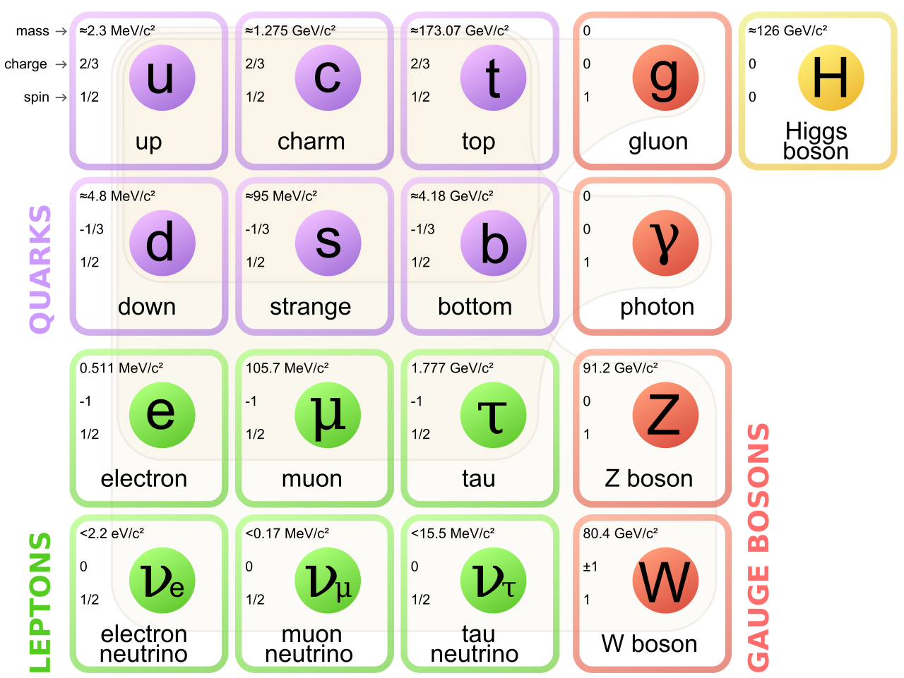So what is it, then? Well… From the table above, you can see that the property of ‘spin’ (i.e. the third number in the top left-hand corner) matches the above-mentioned dichotomy in behavior, i.e. the two different types of interference (bosons versus fermions or, to use a heavier term, Bose-Einstein statistics versus Fermi-Dirac statistics): all matter-particles are so-called spin-1/2 particles, while all force-carriers (gauge bosons) all have spin one. [Never mind the Higgs particle: that’s ‘just’ a mechanism to give (most) elementary particles some mass.]

So why is that? Why are matter-particles spin-1/2 particles and force-carries spin-1 particles? To answer that question, we need to answer the question: what’s this spin number? And to answer that question, we first need to answer the question: what’s spin?

Spin in the classical world

In the classical world, it’s, quite simply, the momentum associated with a spinning or rotating object, which is referred to as the angular momentum. We’ve analyzed the math involved in another post, and so I won’t dwell on that here, but you should note that, in classical mechanics, we distinguish two types of angular momentum:

1. Orbital angular momentum: that’s the angular momentum an object gets from circling in an orbit, like the Earth around the Sun.
2. Spin angular momentum: that’s the angular momentum an object gets from spinning around its own axis., just like the Earth, in addition to rotating around the Sun, is rotating around its own axis (which is what causes day and night, as you know).

The math involved in both is pretty similar, but it’s still useful to distinguish the two, if only because we’ll distinguish them in quantum mechanics too! Indeed, when I analyzed the math in the above-mentioned post, I showed how we represent angular momentum by a vector that’s perpendicular to the direction of rotation, with its direction given by the ubiquitous right-hand rule—as in the illustration below, which shows both the angular momentum (L) as well as the torque (τ) that’s produced by a rotating mass. The formulas are given too: the angular momentum L is the vector cross product of the position vector r and the linear momentum p, while the magnitude of the torque τ is given by the product of the length of the lever arm and the applied force. An alternative approach is to define the angular velocity ω and the moment of inertia I, and we get the same result: L = Iω. 

Of course, the illustration above shows orbital angular momentum only and, as you know, we no longer have a ‘planetary model’ (aka the Rutherford model) of an atom. So should we be looking at spin angular momentum only?

Well… Yes and no. More yes than no, actually. But it’s ambiguous. In addition, the analogy between the concept of spin in quantum mechanics, and the concept of spin in classical mechanics, is somewhat less than straightforward. Well… It’s not straightforward at all actually. But let’s get on with it and use more precise language. Let’s first explore it for light, not because it’s easier (it isn’t) but… Well… Just because. 🙂

The spin of a photon

I talked about the polarization of light in previous posts (see, for example, my post on vector analysis): when we analyze light as a traveling electromagnetic wave (so we’re still in the classical analysis here, not talking about photons as ‘light particles’), we know that the electric field vector oscillates up and down and is, in fact, likely to rotate in the xy-plane (with z being the direction of propagation). The illustration below shows the idealized (aka limiting) case of perfectly circular polarization: if there’s polarization, it is more likely to be elliptical. The other limiting case is plane polarization: in that case, the electric field vector just goes up and down in one direction only. [In case you wonder whether ‘real’ light is polarized, it often is: there’s an easy article on that on the Physics Classroom site.]

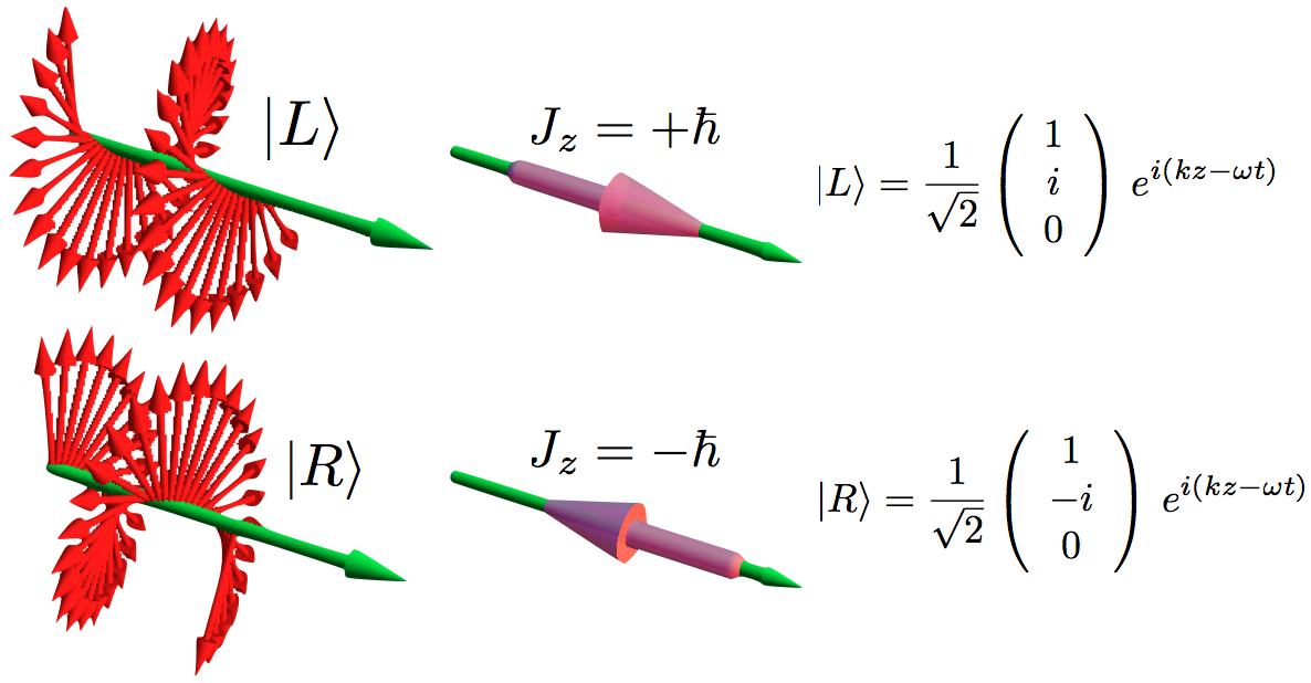The illustration above uses Dirac’s bra-ket notation |L〉 and |R〉 to distinguish the two possible ‘states’, which are left- or right-handed polarization respectively. In case you forgot about bra-ket notations, let me quickly remind you: an amplitude is usually denoted by 〈x|s〉, in which 〈x| is the so-called ‘bra’, i.e. the final condition, and |s〉 is the so-called ‘ket’, i.e. the starting condition, so 〈x|s〉 could mean: a photon leaves at s (from source) and arrives at x. It doesn’t matter much here. We could have used any notation, as we’re just describing some state, which is either |L〉 (left-handed polarization) or |R〉 (right-handed polarization). The more intriguing extras in the illustration above, besides the formulas, are the values: ± ħ = ±h/2π. So that’s plus or minus the (reduced) Planck constant which, as you know, is a very tiny constant. I’ll come back to that. So what exactly is being represented here?

At first, you’ll agree it looks very much like the momentum of light (p) which, in a previous post, we calculated from the (average) energy (E) as p = E/c. Now, we know that E is related to the (angular) frequency of the light through the Planck-Einstein relation E = hν = ħω. Now, ω is the speed of light (c) times the wave number (k), so we can write: p = ħω = ħck/c = ħk. The wave number is the ‘spatial frequency’, expressed either in cycles per unit distance (1/λ) or, more usually, in radians per unit distance (k = 2π/λ), so we can also write p = ħk = h/λ. Whatever way we write it, we find that this momentum (p) depends on the energy and/or, what amounts to saying the same, the frequency and/or the wavelength of the light.

So… Well… The momentum of light is not just h or ħ, i.e. what’s written in that illustration above. So it must be something different. In addition, I should remind you this momentum was calculated from the magnetic field vector, as shown below (for more details, see my post on vector calculus once again), so it had nothing to do with polarization really.

Finally, last but not least, the dimensions of ħ and p = h/λ are also different (when one is confused, it’s always good to do a dimensional analysis in physics):

1. The dimension of Planck’s constant (both h as well as ħ = h/2π) is energy multiplied by time (J·s or eV·s) or, equivalently, momentum multiplied by distance. It’s referred to as the dimension of action in physics, and h is effectively, the so-called quantum of action.
2. The dimension of (linear) momentum is… Well… Let me think… Mass times velocity (mv)… But what’s the mass in this case? Light doesn’t have any mass. However, we can use the mass-energy equivalence: 1 eV = 1.7826×10⁻³⁶ kg. [10⁻³⁶? Well… Yes. An electronvolt is a very tiny measure of energy.] So we can express p in eV·m/s units.

Hmm… We can check: momentum times distance gives us the dimension of Planck’s constant again – (eV·m/s)·m = eV·s. OK. That’s good… […] But… Well… All of this nonsense doesn’t make us much smarter, does it? 🙂 Well… It may or may not be more useful to note that the dimension of action is, effectively, the same as the dimension of angular momentum. Huh? Why? Well… From our classical L = r×p formula, we find L should be expressed in m·(eV·m/s) = eV·m²/s  units, so that’s… What? Well… Here we need to use a little trick and re-express energy in mass units. We can then write L in kg·m²/s units and, because 1 Newton (N) is 1 kg⋅m/s², the kg·m²/s unit is equivalent to the N·m·s = J·s unit. Done!

Having said that, all of this still doesn’t answer the question: are the linear momentum of light, i.e. our p, and those two angular momentum ‘states’, |L〉 and |R〉, related? Can we relate |L〉 and |R〉 to that L = r×p formula?

The answer is simple: no. The |L〉 and |R〉 states represent spin angular momentum indeed, while the angular momentum we would derive from the linear momentum of light using that L = r×p is orbital angular momentum. Let’s introduce the proper symbols: orbital angular momentum is denoted by L, while spin angular momentum is denoted by S. And then the total angular momentum is, quite simply, J = L + S.

L and S can both be calculated using either a vector cross product r × p (but using different values for r and p, of course) or, alternatively, using the moment of inertia tensor I and the angular velocity ω. The illustrations below (which I took from Wikipedia) show how, and also shows how L and S are added to yield J = L + S.

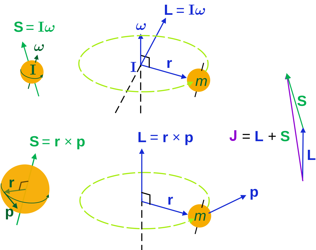
So what? Well… Nothing much. The illustration above show that the analysis – which is entirely classical, so far – is pretty complicated. [You should note, for example, that in the S = Iω and L = Iω formulas, we don’t use the simple (scalar) moment of inertia but the moment of inertia tensor (so that’s a matrix denoted by I, instead of the scalar I), because S (or L) and ω are not necessarily pointing in the same direction.

By now, you’re probably very confused and wondering what’s wiggling really. The answer for the orbital angular momentum is: it’s the linear momentum vector p. Now…

Hey! Stop! Why would that vector wiggle?

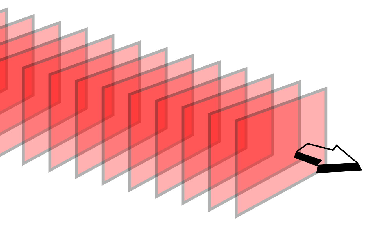
You’re right. Perhaps it doesn’t. The linear momentum p is supposed to be directed in the direction of travel of the wave, isn’t it? It is. In vector notation, we have p = ħk, and that k vector (i.e. the wavevector) points in the direction of travel of the wave indeed and so… Well… No. It’s not that simple. The wave vector is perpendicular to the surfaces of constant phase, i.e. the so-called wave fronts, as show in the illustration below (see the direction of e_k, which is a unit vector in the direction of k).

So, yes, if we’re analyzing light moving in a straight one-dimensional line only, or we’re talking a plane wave, as illustrated below, then the orbital angular momentum vanishes.

But the orbital angular momentum L does not vanish when we’re looking at a real light beam, like the ones below. Real waves? Well… OK… The ones below are idealized wave shapes as well, but let’s say they are somewhat more real than a plane wave. 🙂

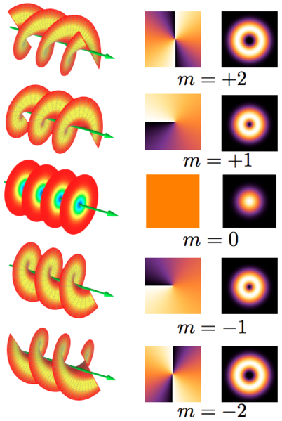
So what do we have here? We have wavefronts that are shaped as helices, except for the one in the middle (marked by m = 0) which is, once again, an example of plane wave—so for that one (m = 0), we have zero orbital angular momentum indeed. But look, very carefully, at the m = ± 1 and m = ± 2 situations. For m = ± 1, we have one helical surface with a step length equal to the wavelength λ. For m = ± 2, we have two intertwined helical surfaces with the step length of each helix surface equal to 2λ. [Don’t worry too much about the second and third column: they show a beam cross-section (so that’s not a wave front but a so-called phase front) and the (averaged) light intensity, again of a beam cross-section.] Now, we can further generalize and analyze waves composed of m helices with the step length of each helix surface equal to |m|λ. The Wikipedia article on OAM (orbital angular momentum of light), from which I got this illustration, gives the following formula to calculate the OAM:

The same article also notes that the quantum-mechanical equivalent of this formula, i.e. the orbital angular momentum of the photons one would associate with the not-cylindrically-symmetric waves above (i.e. all those for which m ≠ 0), is equal to:

L_z = mħ

So what? Well… I guess we should just accept that as a very interesting result. For example, I duly note that L_z is along the direction of propagation of the wave (as indicated by the z subscript), and I also note the very interesting fact that, apparently, L_z  can be either positive or negative. Now, I am not quite sure how such result is consistent with the idea of radiation pressure, but I am sure there must be some logical explanation to that. The other point you should note is that, once again, any reference to the energy (or to the frequency or wavelength) of our photon has disappeared. Hmm… I’ll come back to this, as I promised above already.

The thing is that this rather long digression on orbital angular momentum doesn’t help us much in trying to understand what that spin angular momentum (SAM) is all about. So, let me just copy the final conclusion of the Wikipedia article on the orbital angular momentum of light: the OAM is the component of angular momentum of light that is dependent on the field spatial distribution, not on the polarization of light.

So, again, what’s the spin angular momentum? Well… The only guidance we have is that same little drawing again and, perhaps, another illustration that’s supposed to compare SAM with OAM (underneath).

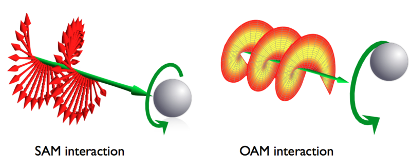Now, the Wikipedia article on SAM (spin angular momentum), from which I took the illustrations above, gives a similar-looking formula for it:

When I say ‘similar-looking’, I don’t mean it’s the same. [Of course not! Spin and orbital angular momentum are two different things!]. So what’s different in the two formulas? Well… We don’t have any del operator (∇) in the SAM formula, and we also don’t have any position vector (r) in the integral kernel (or integrand, if you prefer that term). However, we do find both the electric field vector (E) as well as the (magnetic) vector potential (A) in the equation again. Hence, the SAM (also) takes both the electric as well as the magnetic field into account, just like the OAM. [According to the author of the article, the expression also shows that the SAM is nonzero when the light polarization is elliptical or circular, and that it vanishes if the light polarization is linear, but I think that’s much more obvious from the illustration than from the formula… However, I realize I really need to move on here, because this post is, once again, becoming way too long. So…]

OK. What’s the equivalent of that formula in quantum mechanics?

Well… In quantum mechanics, the SAM becomes a ‘quantum observable’, described by a corresponding operator which has only two eigenvalues:

S_z = ± ħ

So that corresponds to the two possible values for J_z, as mentioned in the illustration, and we can understand, intuitively, that these two values correspond to two ‘idealized’ photons which describe a left- and right-handed circularly polarized wave respectively.

So… Well… There we are. That’s basically all there is to say about it. So… OK. So far, so good.

But… Yes? Why do we call a photon a spin-one particle?

That has to do with convention. A so-called spin-zero particle has no degrees of freedom in regard to polarization. The implied ‘geometry’ is that a spin-zero particle is completely symmetric: no matter in what direction you turn it, it will always look the same. In short, it really behaves like a (zero-dimensional) mathematical point. As you can see from the overview of all elementary particles, it is only the Higgs boson which has spin zero. That’s why the Higgs field is referred to as a scalar field: it has no direction. In contrast, spin-one particles, like photons, are also ‘point particles’, but they do come with one or the other kind of polarization, as evident from all that I wrote above. To be specific, they are polarized in the xy-plane, and can have one of two directions. So, when rotating them, you need a full rotation of 360° if you want them to look the same again.

Now that I am here, let me exhaust the topic (to a limited extent only, of course, as I don’t want to write a book here) and mention that, in theory, we could also imagine spin-2 particles, which would look the same after half a rotation (180°). However, as you can see from the overview, none of the elementary particles has spin-2. A spin-2 particle could be like some straight stick, as that looks the same even after it is rotated 180 degrees. I am mentioning the theoretical possibility because the graviton, if it would effectively exist, is expected to be a massless spin-2 boson. [Now why do I mention this? Not sure. I guess I am just noting this to remind you of the fact that the Higgs boson is definitely not the (theoretical) graviton, and/or that we have no quantum theory for gravity.]

Oh… That’s great, you’ll say. But what about all those spin-1/2 particles in the table? You said that all matter-particles are spin 1/2 particles, and that it’s this particular property that actually makes them matter-particles. So what’s the geometry here? What kind of ‘symmetries’ do they respect?

Well… As strange as it sounds, a spin-1/2 particle needs two full rotations (2×360°=720°) until it is again in the same state. Now, in regard to that particularity, you’ll often read something like: “There is nothing in our macroscopic world which has a symmetry like that.” Or, worse, “Common sense tells us that something like that cannot exist, that it simply is impossible.” [I won’t quote the site from which I took this quotes, because it is, in fact, the site of a very respectable  research center!] Bollocks! The Wikipedia article on spin has this wonderful animation: look at how the spirals flip between clockwise and counterclockwise orientations, and note that it’s only after spinning a full 720 degrees that this ‘point’ returns to its original configuration after spinning a full 720 degrees.

So, yes, we can actually imagine spin-1/2 particles, and with not all that much imagination, I’d say. But… OK… This is all great fun, but we have to move on. So what’s the ‘spin’ of these spin-1/2 particles and, more in particular, what’s the concept of ‘spin’ of an electron?

The spin of an electron

When starting to read about it, I thought that the angular momentum of an electron would be easier to analyze than that of a photon. Indeed, while a photon has no mass and no electric charge, that analysis with those E and B vectors is damn complicated, even when sticking to a strictly classical analysis. For an electron, the classical picture seems to be much more straightforward—but only at first indeed. It quickly becomes equally weird, if not more.

We can look at an electron in orbit as a rotating electrically charged ‘cloud’ indeed. Now, from Maxwell’s equations (or from your high school classes even), you know that a rotating electric charged body creates a magnetic dipole. So an electron should behave just like a tiny bar magnet. Of course, we have to make certain assumptions about the distribution of the charge in space but, in general, we can write that the magnetic dipole moment μ is equal to:

In case you want to know, in detail, where this formula comes from, let me refer you to Feynman once again, but trust me – for once 🙂 – it’s quite straightforward indeed: the L in this formula is the angular momentum, which may be the spin angular momentum, the orbital angular momentum, or the total angular momentum. The e and m are, of course, the charge and mass of the electron respectively.

So that’s a good and nice-looking formula, and it’s actually even correct except for the spin angular momentum as measured in experiments. [You’ll wonder how we can measure orbital and spin angular momentum respectively, but I’ll talk about an 1921 experiment in a few minutes, and so that will give you some clue as to that mystery. :-)] To be precise, it turns out that one has to multiply the above formula for μ with a factor which is referred to as the g-factor. [And, no, it’s got nothing to do with the gravitational constant or… Well… Nothing. :-)] So, for the spin angular momentum, the formula should be:

Experimental physicists are constantly checking that value and they know measure it to be something like g = is 2.00231930419922 ± 1.5×10⁻¹². So what’s the explanation for that g? Where does it come from? There is, in fact, a classical explanation for it, which I’ll copy hereunder (yes, from Wikipedia). This classical explanation is based on assuming that the distribution of the electric charge of the electron and its mass does not coincide:

Why do I mention this classical explanation? Well… Because, in most popular books on quantum mechanics (including Feynman’s delightful QED), you’ll read that (a) the value for g can be derived from a quantum-theoretical equation known as Dirac’s equation (or ‘Dirac theory’, as it’s referred to above) and, more importantly, that (b) physicists call the “accurate prediction of the electron g-factor” from quantum theory (i.e. ‘Dirac’s theory’ in this case) “one of the greatest triumphs” of the theory.

So what about it? Well… Whatever the merits of both explanations (classical or quantum-mechanical), they are surely not the reason why physicists abandoned the classical theory. So what was the reason then? What a stupid question! You know that already! The Rutherford model was, quite simply, not consistent: according to classical theory, electrons should just radiate their energy away and spiral into the nucleus. More in particular, there was yet another experiment that wasn’t consistent with classical theory, and it’s one that’s very relevant for the discussion at hand: it’s the so-called Stern-Gerlach experiment.

It was just as ‘revolutionary’ as the Michelson-Morley experiment (which couldn’t measure the speed of light), or the discovery of the positron in 1932. The Stern-Gerlach experiment was done in 1921, so that’s many years before quantum theory replaced classical theory and, hence, it’s not one of those experiments confirming quantum theory. No. Quite the contrary. It was, in fact, one of the experiments that triggered the so-called quantum revolution. Let me insert the experimental set-up and summarize it (below).

• The German scientists Otto Stern and Walther Gerlach produced a beam of electrically-neutral silver atoms and let it pass through a (non-uniform) magnetic field. Why silver atoms? Well… Silver atoms are easy to handle (in a lab, that is) and easy to detect with a photoplate.
• These atoms came out of an oven (literally), in which the silver was being evaporated (yes, one can evaporate silver), so they had no special orientation in space and, so Stern and Gerlach thought, the magnetic moment (or spin) of the outer electrons in these atoms would point into all possible directions in space.
• As expected, the magnetic field did deflect the silver atoms, just like it would deflect little dipole magnets if you would shoot them through the field. However, the pattern of deflection was not the one which they expected. Instead of hitting the plate all over the place, within some contour, of course, only the contour itself was hit by the atoms. There was nothing in the middle!
• And… Well… It’s a long story, but I’ll make it short. There was only one possible explanation for that behavior, and that’s that the magnetic moments – and, therefore the spins – had only two orientations in space, and two possible values only which – Surprise, surprise! – are ±ħ/2 (so that’s half the value of the spin angular momentum of photons, which explains the spin-1/2 terminology).

The spin angular momentum of an electron is more popularly known as ‘up’ or ‘down’.

So… What about it? Well… It explains why a atomic orbital can have two electrons, rather than one only and, as such, the behavior of the electron here is the basis of the so-called periodic table, which explains all properties of the chemical elements. So… Yes. Quantum theory is relevant, I’d say. 🙂

Conclusion

This has been a terribly long post, and you may no longer remember what I promised to do. What I promised to do, is to write some more about the difference between a photon and an electron and, more in particular, I said I’d write more about their charge, and that “weird number”: their spin. I think I lived up to that promise. The summary is simple:

1. Photons have no (electric) charge, but they do have spin. Their spin is linked to their polarization in the xy-plane (if z is the direction of propagation) and, because of the strangeness of quantum mechanics (i.e. the quantization of (quantum) observables), the value for this spin is either +ħ or –ħ, which explains why they are referred to as spin-one particles (because either value is one unit of the Planck constant).
2. Electrons have both electric charge as well as spin. Their spin is different and is, in fact, related to their electric charge. It can be interpreted as the magnetic dipole moment, which results from the fact we have a spinning charge here. However, again, because of the strangeness of quantum mechanics, their dipole moment is quantized and can take only one of two values: ±ħ/2, which is why they are referred to as spin-1/2 particles.

So now you know everything you need to know about photons and electrons, and then I mean real photons and electrons, including their properties of charge and spin. So they’re no longer ‘fake’ spin-zero photons and electrons now. Isn’t that great? You’ve just discovered the real world! 🙂

So… I am done—for the moment, that is… 🙂 If anything, I hope this post shows that even those ‘weird’ quantum numbers are rooted in ‘physical reality’ (or in physical ‘geometry’ at least), and that quantum theory may be ‘crazy’ indeed, but that it ‘explains’ experimental results. Again, as Feynman says:

“We understand how Nature works, but not why Nature works that way. Nobody understands that. I can’t explain why Nature behave in this particular way. You may not like quantum theory and, hence, you may not accept it. But physicists have learned to realize that whether they like a theory or not is not the essential question. Rather, it is whether or not the theory gives predictions that agree with experiment. The theory of quantum electrodynamics describes Nature as absurd from the point of view of common sense. But it agrees fully with experiment. So I hope you can accept Nature as She is—absurd.”

Frankly speaking, I am not quite prepared to accept Nature as absurd: I hope that some more familiarization with the underlying mathematical forms and shapes will make it look somewhat less absurd. More, I hope that such familiarization will, in the end, make everything look just as ‘logical’, or ‘natural’ as the two ways in which amplitudes can ‘interfere’.

Post scriptum: I said I would come back to the fact that, in the analysis of orbital and spin angular momentum of a photon (OAM and SAM), the frequency or energy variable sort of ‘disappears’. So why’s that? Let’s look at those expressions for |L〉 and |R〉 once again:

What’s written here really? If |L〉 and |R〉 are supposed to be equal to either +ħ or –ħ, then that product of e^i(kz–ωt) with the 3×1 matrix (which is a ‘column vector’ in this case) does not seem to make much sense, does it? Indeed, you’ll remember that e^i(kz–ωt) just a regular wave function. To be precise, its phase is φ = kz–ωt (with z the direction of propagation of the wave), and its real and imaginary part can be written as e^iφ = cos(φ) + isin(φ) = a + bi. Multiplying it with that 3×1 column vector (1, i, 0) or (1, –i, 0) just yields another 3×1 column vector. To be specific, we get:

1. The 3×1 ‘vector’ (a + bi, –b+ai, 0) for |L〉, and
2. The 3×1 ‘vector’ (a + bi, b–ai, 0) for |R〉.

So we have two new ‘vectors’ whose components are complex numbers. Furthermore, we can note that their ‘x’-component is the same, their ‘y’-component is each other’s opposite –b+ai = –(b–ai), and their ‘z’-component is 0.

So… Well… In regard to their ‘y’-component, I should note that’s just the result of the multiplication with i and/or –i: multiplying a complex number with i amounts to a 90° degree counterclockwise rotation, while multiplication with –i amounts to the same but clockwise. Hence, we must arrive at two complex numbers that are each other’s opposite. [Indeed, in complex analysis, the value –1 = e^iπ = e^–iπ is a 180° rotation, both clockwise (φ = –π) or counterclockwise (φ = +π), of course!.]

Hmm… Still… What does it all mean really? The truth is that it takes some more advanced math to interpret the result. To be precise, pure quantum states, such |L〉 and |R〉 here, are represented by so-called ‘state vectors’ in a Hilbert space over complex numbers. So that’s what we’ve got here. So… Well… I can’t say much more about this right now: we’ll just need to study some more before we’ll ‘understand’ those expressions for |L〉 and |R〉. So let’s not worry about it right now. We’ll get there.

Just for the record, I should note that, initially, I thought 1/√2 factor in front gave some clue as to what’s going on here: 1/√2 ≈ 0.707 is a factor that’s used to calculate the root mean square (RMS) value for a sine wave. It’s illustrated below. The RMS value is a ‘special average’ one can use to calculate the energy or power (i.e. energy per time unit) of a wave. [Using the term ‘average’ is misleading, because the average of a sine wave is 1/2 over half a cycle, and 0 over a fully cycle, as you can easily see from the shape of the function. But I guess you know what I mean.]

Indeed, you’ll remember that the energy (E) of a wave is proportional to the square of its amplitude (A): E ∼ A². For example, when we have a constant current I, the power P will be proportional to its square: P ∼ I². With a varying current (I) and voltage (V), the formula is more complicated but we can simply it using the rms values: P_avg = V_RMS·I_RMS.

So… Looking at that formula, should we think of h and/or ħ as some kind of ‘average’ energy, like the energy of a photon per cycle or per radian? That’s an interesting idea so let’s explore it. If the energy of a photon is equal to E = h·ν = h·ω/2π = ħω, then we can also write:

h = E/ν and/or ħ = E/ω

So, yes: h is the energy of a photon per cycle obviously and, because the phase covers 2π radians during each cycle, and ħ must be the energy of the photon per radian! That’s a great result, isn’t it? It also gives a wonderfully simple interpretation to Planck’s quantum of action!

Well… No. We made at least two mistakes here. The first mistake is that if we think of a photon as wave train being radiated by an atom – which, as we calculated in another post, lasts about 3.2×10^–8 seconds – the graph for its energy is going to resemble the graph of its amplitude, so it’s going to die out and each oscillation will carry less and less energy. Indeed, the decay time given here (τ = 3.2×10^–8 seconds) was the time it takes for the radiation (we assumed sodium light with a wavelength of 600 nanometer) to die out by a factor 1/e. To be precise, the shape of the energy curve is E = E₀e^−t/τ, and so it’s an envelope resembling the A(t) curve below.

Indeed, remember, the energy of a wave is determined not only by its frequency (or wavelength) but also by its amplitude, and so we cannot assume the amplitude of a ‘photon wave’ is going to be the same everywhere. Just for the record: note that the energy of a wave is proportional to the frequency (doubling the frequency doubles the energy) but, when linking it to the amplitude, we should remember that the energy is proportional to the square of the amplitude, so we write E ∼ A².

The second mistake is that both ν and ω are the light frequency (expressed in cycles or radians respectively) of the light per second, i.e per time unit. So that’s not the number of cycles or radians that we should associate with the wavetrain! We should use the number of cycles (or radians) packed into one photon. We can calculate that easily from the value for the decay time τ. Indeed, for sodium light, which which has a frequency of 500 THz (500×10¹² oscillations per second) and a wavelength of 600 nm (600×10^–9 meter), we said the radiation lasts about 3.2×10^–8 seconds (that’s actually the time it takes for the radiation’s energy to die out by a factor 1/e, so the wavetrain will actually last (much) longer, but so the amplitude becomes quite small after that time), and so that makes for some 16 million oscillations, and a ‘length’ of the wavetrain of about 9.6 meter! Now, the energy of a sodium light photon is about 2eV (h·ν ≈ 4×10⁻¹⁵ electronvolt·second times 0.5×10¹⁵ cycles/sec = 2eV) and so we could say the average energy of each of those 16 million oscillations would be 2/(16×10⁶) eV = 0.125×10^–6 eV. But, from all that I wrote above, it’s obvious that this number doesn’t mean all that much, because the wavetrain is not likely to be shaped very regularly.

So, in short, we cannot say that h is the photon energy per cycle or that ħ is the photon energy per radian!  That’s not only simplistic but, worse, false. Planck’s constant is what is is: a factor of proportionality for which there is no simple ‘arithmetic’ and/or ‘geometric’ explanation. It’s just there, and we’ll need to study some more math to truly understand the meaning of those two expressions for |L〉 and |R〉.

Having said that, and having thought about it all some more, I find there’s, perhaps, a more interesting way to re-write E = h·ν:

h = E/ν = (λ/c)E = T·E

T? Yes. T is the period, so that’s the time needed for one oscillation: T is just the reciprocal of the frequency (T = 1/ν = λ/c). It’s a very tiny number, because we divide (1) a very small number (the wavelength of light measured in meter) by (2) a very large number (the distance (in meter) traveled by light). For sodium light, T is equal to 2×10^–15 seconds, so that’s two femtoseconds, i.e. two quadrillionths of a second.

Now, we can think of the period as a fraction of a second, and smaller fractions are, obviously, associated with higher frequencies and, what amounts to the same, shorter wavelengths (and, hence, higher energies). However, when writing T = λ/c, we can also think of T being another kind of fraction: λ/c can also be written as the ratio of the wavelength and the distance traveled by light in one second, i.e. a light-second (remember that light-seconds are measures of length, not of distance). The two fractions are the same when we express time and distance in equivalent units indeed (i.e. distance in light-second, or time in sec/c units).

So that links h to both time as well as distance and we may look at h as some kind of fraction or energy ‘density’ even (although the term ‘density’ in this context is not quite accurate). In the same vein, I should note that, if there’s anything that should make you think about h, is the fact that its value depends on how we measure time and distance. For example, if w’d measure time in other units (for example, the more ‘natural’ unit defined by the time light needs to travel one meter), then we get a different unit for h. And, of course, you also know we can relate energy to distance (1 J = 1 N·m). But that’s something that’s obvious from h‘s dimension (J·s), and so I shouldn’t dwell on that.

Hmm… Interesting thoughts. I think I’ll develop these things a bit further in one of my next posts. As for now, however, I’ll leave you with your own thoughts on it.

Note 1: As you’re trying to follow what I am writing above, you may have wondered whether or not the duration of the wavetrain that’s emitted by an atom is a constant, or whether or not it packs some constant number of oscillations. I’ve thought about that myself as I wrote down the following formula at some point of time:

h = (the duration of the wave)·(the energy of the photon)/(the number of oscillations in the wave)

As mentioned above, interpreting h as some kind of average energy per oscillation is not a great idea but, having said that, it would be a good exercise for you to try to answer that question in regard to the duration of these wavetrains, and/or the number of oscillations packed into them, yourself. There are various formulas for the Q of an atomic oscillator, but the simplest one is the one expressed in terms of the so-called classical electron radius r₀:

Q = 3λ/4πr₀

As you can see, the Q depends on λ: higher wavelengths (so lower energy) are associated with higher Q. In fact, the relationship is directly proportional: twice the wavelength will give you twice the Q. Now, the formula for the decay time τ is also dependent on the wavelength. Indeed, τ = 2Q/ω = Qλ/πc. Combining the two formulas yields (if I am not mistaken):

τ = 3λ²/4π²r₀c.

Hence, the decay time is proportional to the square of the wavelength. Hmm… That’s an interesting result. But I really need to learn how to be a bit shorter, and so I’ll really let you think now about what all this means or could mean.

Note 2: If that 1/√2 factor has nothing to do with some kind of rms calculation, where does it come from? I am not sure. It’s related to state vector math, it seems, and I haven’t started that as yet. I just copy a formula from Wikipedia here, which shows the same factor in front:

The formula above is said to represent the “superposition of joint spin states for two particles”. My gut instinct tells me 1/√2 factor has to do with the normalization condition and/or with the fact that we have to take the (absolute) square of the (complex-valued) amplitudes to get the probability.

Some content on this page was disabled on June 17, 2020 as a result of a DMCA takedown notice from Michael A. Gottlieb, Rudolf Pfeiffer, and The California Institute of Technology. You can learn more about the DMCA here:

https://en.support.wordpress.com/copyright-and-the-dmca/
Some content on this page was disabled on June 17, 2020 as a result of a DMCA takedown notice from Michael A. Gottlieb, Rudolf Pfeiffer, and The California Institute of Technology. You can learn more about the DMCA here:

https://en.support.wordpress.com/copyright-and-the-dmca/