Magnetostatics: the vector potential

This and the next posts are supposed to wrap up a few loose ends on magnetism. One of these loose ends is the (magnetic) vector potential, which we introduced in our post on gauge transformations, but then we didn’t do much with it. Another topic I neglected so far is that of the magnetic dipole moment (as opposed to the electric dipole moment), which is an extremely important concept both in classical as well as in quantum mechanics. So let’s do the vector potential here, and the magnetic dipole moment in the next. 🙂

Let’s go for it. Let me recall the basics which, as usual, are just Maxwell’s equations. You’ll remember that the electrostatic field was curl-free: ∇×E = 0, everywhere. Therefore, we can apply the following mathematical theorem: if the curl of a vector field is zero (everywhere), then the vector field can be represented as the gradient of some scalar function:

if ∇×C = 0, then there is some Ψ for which C = ∇Ψ

Substituting C for E, and taking into account our conventions on charge and the direction of flow, we wrote:

E = –∇Φ

Φ (phi) is referred to as the electric potential. Combining E = –∇Φ with Gauss’ Law – ∇•E = ρ/ε₀ − we got Poisson’s equation:

∇²Φ = −ρ/ε₀

So that equation sums up all of electrostatics. Really: that’s it! 🙂

Now, the two equations for magnetostatics are: ∇•B = 0 and c²∇×B = j/ε₀. Let me say something more about them:

1. The ∇•B = 0 equation is true, always, unlike the ∇×E = 0 expression, which is true for electrostatics only (no moving charges).
2. The ∇•B = 0 equation says the divergence of B is zero, always. Now, you can verify for yourself that the divergence of the curl of a vector field is always zero, so div (curl A) = ∇•(∇×A) = 0, always. Therefore, there’s another theorem that we can apply. It says the following: if the divergence of a vector field, say D, is zero – so if ∇•D = 0, then D will be the the curl of some other vector field C, so we can write: D = ∇×C.  Applying this to ∇•B = 0, we can write: 

If ∇•B = 0, then there is an A such that B = ∇×A

We can also write this as follows: ∇·B = ∇·(∇×A) = 0 and, hence, B = ∇×A. Now, it’s this vector field A that is referred to as the (magnetic) vector potential, and so that’s what we want to talk about here. As a start, it may be good to write all of the components of our B = ∇×A vector:

Note that we have no ‘time component’ because we assume the fields are static, so they do not change with time. Now, because that’s a relatively simple situation, you may wonder whether we really simplified anything with this vector potential. B is a vector with three components, and so is A. The answer to that question is somewhat subtle, and similar to what we did for electrostatics: it’s mathematically convenient to use A, and then calculate the derivatives above to find B. So the number of components doesn’t matter really: it’s just more convenient to first get A using our data on the currents j, and then we get B from A.

That’s it really. Let me show you how it works. The whole argument is somewhat lengthy, but it’s not difficult, and once it’s done, it’s done. So just carry on and please bear with me 🙂

First, we need to put some constraints on A, because the B = ∇×A equation does not fully define A. It’s like the scalar potential Φ: any Φ’ = Φ + C was as good a choice as Φ (with C any constant), so we needed a reference point Φ = 0, which we usually took at infinity. With the vector potential A, we have even more latitude: we can not only add a constant but any field which is the gradient of some scalar field, so any A’ = A + ∇Ψ will do. Why? Just write it all out: ∇×(A + ∇Ψ) = ∇×A + ∇×(∇Ψ). But the curl of the gradient of a scalar field (or a scalar function) is always zero (you can check my post on vector calculus on this), so ∇×(∇Ψ) = 0 and so ∇×(A + ∇Ψ) = ∇×A + ∇×(∇Ψ) = ∇×A + 0 = ∇×A = B.

So what constraints should we put on our choice of A? The choice is, once again, based on mathematical convenience: in magnetostatics, we’ll choose A such that ∇•A = 0. Can we do that? Yes. The A’ = A + ∇Ψ flexibility allows us to make ∇•A’ anything we wish, and so A and A’ will have the same curl, but they don’t need to have the same divergence. So we can choose an A’ so ∇•A’ = 0, and then we denote A’ by A. 🙂 So our ‘definition’ of the vector potential A is now:

B = ∇×A and ∇•A = 0

I have to make two points here:

1. First, you should note that, in my post on gauges, I mentioned that the choice is different when the time derivatives of E and B are not equal to zero, so when we’re talking changing currents and charge distributions, so that’s dynamics. However, that’s not a concern here.
2. To be fully complete, I should note that the ‘definition’ above does still not uniquely determine A. For a unique specification, we also need some reference point, or say how the field behaves on some boundary, or at large distances. It is usually convenient to choose a field which goes to zero at large distances, just like our electric potential.

Phew! We’ve said so many things about A now, but nothing that has any relevance to how we’d calculate A. 😦 So we are we heading here?

Fortunately, we can go a bit faster now. The c²∇×B = j/ε₀ equation and our B = ∇×A give us:

c²∇×(∇×A) = j/ε₀

Now, there’s this other vector identity, which you surely won’t remember either—but trust me: I am not lying: ∇×(∇×A) = ∇(∇•A) − ∇²A. So, now you see why we choose A such that ∇•A = 0 ! It allows us to write:

c²∇×(∇×A) = − c²∇²A = j/ε₀ ⇔ ∇²A = –j/ε₀c²

Now, the three components of ∇²A = –j/ε₀c² are, of course:

As you can see, each of these three equations is mathematically identical to that Poisson equation: ∇²Φ = − ρ/ε₀. So all that we learned about solving for potentials when ρ is known can now be used to solve for each component of A when j is known. Now, to calculate Φ, we used the following integral:

Simply substituting symbols then gives us the solution for A_x:

We have a similar integral for A_y and A_z, of course, and we can combine the three equations in vector form:

Finally, and just in case you wonder what is what, there’s the illustration below (taken from Feynman’s Lecture on this topic here) that, hopefully, will help you to make sense of it all.

At this point, you’re probably tired of these formulas (or asleep) or (if you’re not asleep) wondering what they mean really, so let’s do two examples. Of course, you won’t be surprised that we’ll be talking a straight wire and a solenoid respectively once again. 🙂

The magnetic field of a straight wire

We already calculated the magnetic field of a straight wire, using Ampère’s Law and the symmetry of the situation, in our previous post on magnetostatics. We got the following formula:

Do we get the same using those formulas for A and then doing our derivations to get B? We should, and we do, but I’ll be lazy here and just refer you to the relevant section in Feynman’s Lecture on it, because the solenoid stuff is much more interesting. 🙂

The magnetic field of a solenoid

In the mentioned post on magnetostatics, we also derived a formula for the magnetic field inside a solenoid. We got:

with n the number of turns per unit length of the solenoid, and I the current going through it. However, in the mentioned post, we assumed that the magnetic field outside of the solenoid was zero, for all practical purposes, but it is not. It is very weak but not zero, as shown below. In fact, it’s fairly strong at very short distances from the solenoid! Calculating the vector potential allows us to calculate its exact value, everywhere. So let’s go for it.

The relevant quantities are shown in the illustration below. So we’ve got a very long solenoid here once again, with n turns of wire per unit length and, therefore, a circumferential current on the surface of n·I per unit length (the slight pitch of the winding is being neglected).

Now, just like that surface charge density ρ in electrostatics, we have a ‘surface current density’ J here, which we define as J = n·I. So we’re going from a scalar to a vector quantity, and the components of J are:

J_x = –J·sinϕ, J_y = –J·cosϕ, J_z = 0

So how do we do this? As should be clear from the whole development above, the principle is that the x-component of the vector potential arising from a current density j is the same as the electric potential Φ that would be produced by a charge density ρ equal to j_x divided by c², and similarly for the y- and z-components. Huh? Yes. Just read it a couple of times and think about it: we should imagine some cylinder with a surface charge ρ = –(J/c²)·sinϕ to calculate A_x. And then we equate ρ with –(J/c²)·cosϕ and zero respectively to find A_y and A_z.  

Now, that sounds pretty easy but Feynman’s argument is quite convoluted here, so I’ll just skip it (click the link here if you’d want to see it) and give you the final result, i.e. the magnitude of A:

Of course, you need to interpret the result above with the illustration, which shows that A is always perpendicular to r’. [In case you wonder why we write r’ (so r with a prime) and not r, that’s to make clear we’re talking the distance from the z-axis, so it’s not the distance from the origin.]

Now, you may think that c² in the denominator explains the very weak field, but it doesn’t: it’s the inverse proportionality to r’ that makes the difference! Indeed, you should compare the formula above with the result we get for the vector potential inside of the solenoid, which is equal to:

The illustration below shows the quantities involved. Note that we’re talking a uniform magnetic field here, along the z-axis, which has the same direction as B₀ and, hence, is pointing towards you as you look at the illustration, which is why you don’t see the B₀ field lines and/or the z-axis: they’re perpendicular to your computer screen, so to speak.

As for the direction of A, it’s shown on the illustration, of course, but let me remind you of the right-hand rule for the vector cross product a×b once again, so you can make sense of the direction of A = (1/2)B₀×r’ indeed:

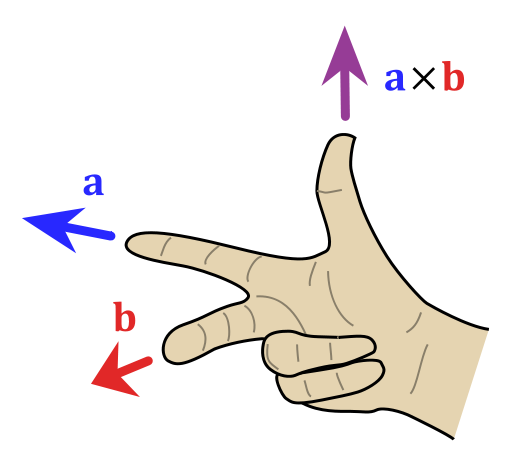Also note the magnitude this formula implies: a×b = |a|·|b|·sinθ·n, with θ the angle between a and b, and n the normal unit vector in the direction given by that right-hand rule above. Now, unlike a vector dot product, the magnitude of the vector cross product is not zero for perpendicular vectors. In fact, when θ = π/2, which is the case for B₀ and r’, then sinθ = 1, and, hence, we can write:

|A| = A = (1/2)|B₀||r’| = (1/2)·B₀·r’

Now, just substitute B₀ for B₀ = n·I/ε₀c², which is the field inside the solenoid, then you get:

A = (1/2)·n·I·r’/ε₀c²

You should compare this formula with the formula for A outside the solenoid, so you can draw the right conclusions. Note that both formulas incorporate the same (1/2)·n·I/ε₀c² factor. The difference, really, is that inside the solenoid, A is proportional to r’ (as shown in the illustration: if r’ doubles, triples etcetera, then A will double, triple etcetera too) while, outside of the solenoid, A is inversely proportional to r’. In addition, outside the solenoid, we have the a² factor, which doesn’t matter inside. Indeed, the radius of the solenoid (i.e. a) changes the flux, which is the product of B and the cross-section area π·a², but not B itself.

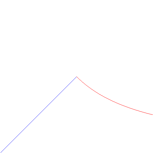
Let’s do a quick check to see if the formula makes sense. We do not want A to be larger outside of the solenoid than inside, obviously, so the a²/r’ factor should be smaller than r’ for r’ > a. Now, a²/r’ < r’ if a² < r’², and because a an r’ are both positive real numbers, that’s the case if r’ > a indeed. So we’ve got something that resembles the electric field inside and outside of a uniformly charged sphere, except that A decreases as 1/r’ rather than as 1/r’², as shown below.

Hmm… That’s all stuff to think about… The thing you should take home from all of this is the following:

1. A (uniform) magnetic field B in the z-direction corresponds to a vector potential A that rotates about the z-axis with magnitude A = B₀·r’/2 (with r’ the displacement from the z-axis, not from the origin—obviously!). So that gives you the A inside of a solenoid. The magnitude is A = (1/2)·n·I·r’/ε₀c², so A is proportional with r’.
2. Outside of the solenoid, A‘s magnitude (i.e. A) is inversely proportional to the distance r’, and it’s given by the formula: A = (1/2)·n·I·a²/ε₀c²·r’. That’s, of course, consistent with the magnetic field diminishing with distance there. But remember: contrary to what you’ve been taught or what you often read, it is not zero. It’s only near zero if r’ >> a.

Alright. Done. Next post. So that’s on the magnetic dipole moment 🙂

Some content on this page was disabled on June 16, 2020 as a result of a DMCA takedown notice from The California Institute of Technology. You can learn more about the DMCA here:

https://wordpress.com/support/copyright-and-the-dmca/
Some content on this page was disabled on June 16, 2020 as a result of a DMCA takedown notice from The California Institute of Technology. You can learn more about the DMCA here:

https://wordpress.com/support/copyright-and-the-dmca/
Some content on this page was disabled on June 16, 2020 as a result of a DMCA takedown notice from The California Institute of Technology. You can learn more about the DMCA here:

https://wordpress.com/support/copyright-and-the-dmca/
Some content on this page was disabled on June 16, 2020 as a result of a DMCA takedown notice from The California Institute of Technology. You can learn more about the DMCA here:

https://wordpress.com/support/copyright-and-the-dmca/
Some content on this page was disabled on June 16, 2020 as a result of a DMCA takedown notice from The California Institute of Technology. You can learn more about the DMCA here:

https://wordpress.com/support/copyright-and-the-dmca/
Some content on this page was disabled on June 16, 2020 as a result of a DMCA takedown notice from The California Institute of Technology. You can learn more about the DMCA here:

https://wordpress.com/support/copyright-and-the-dmca/
Some content on this page was disabled on June 16, 2020 as a result of a DMCA takedown notice from The California Institute of Technology. You can learn more about the DMCA here:

https://wordpress.com/support/copyright-and-the-dmca/
Some content on this page was disabled on June 16, 2020 as a result of a DMCA takedown notice from The California Institute of Technology. You can learn more about the DMCA here:

https://wordpress.com/support/copyright-and-the-dmca/