One of the great pleasures of rereading Feynman’s Lectures is that one occasionally encounters a chapter that feels less like a finished scientific theory and more like a group of brilliant people desperately trying to make sense of an increasingly unruly universe.
The discussion of strangeness in Feynman’s Lecture on what was then (1963-1965) referred to as ‘K-mesons’ (now usually referenced by the portmanteau ‘kaons’, see: Feynman’s Lectures, Vol. III-11-5) is one such chapter.
The historical problem was simple enough.
Physicists had discovered a collection of particles that behaved in very peculiar ways. Certain reactions occurred. Other reactions seemed forbidden. Particles were produced in pairs but decayed individually. Nothing appeared to make sense.
So what did physicists do?
They did what physicists have always done.
They invented a quantum number.
The new quantity was called strangeness.
And, to be fair, it worked remarkably well. The new bookkeeping system immediately organized a bewildering collection of observations into a coherent pattern. Success. Problem solved.
Or was it?
The Department Is Created
Let us imagine an alternative history.
A new particle is discovered.
The Director of the Institute for Advanced Particle Nomenclature immediately convenes an emergency meeting.
“Can we explain it?” asks the Director.
“No,” replies the staff.
“Can we calculate it?”
“Also no.”
“Can we classify it?”
“Absolutely.”
The Director smiles.
A new quantum number is born.
Funding is renewed.
The particle acquires a place in the table.
Order has been restored.
The Conservation Crisis
Several years later, a graduate student bursts into the Director’s office.
“Professor! The particle appears to violate the conservation law!” The Director looks horrified.
“Impossible. The conservation law is conserved.”
“But we’ve observed the violation.”
A long silence follows.
Eventually, a senior professor clears his throat: “The conservation law is approximately conserved.”
Relief spreads throughout the room.
Tea is served.
Several papers are published.
The Great Expansion
Over time, additional anomalies appear. The Institute responds with admirable efficiency. New quantum numbers are introduced.
Strangeness.
Charm.
Color.
Flavor.
Hyperflavor.
Metaflavor.
Administrative Flavor.
Contextual Hyper-Strangeness.
A separate committee is established to study the interactions between Contextual Hyper-Strangeness and Administrative Flavor under conditions of Spontaneous Meta-Symmetry Deconstruction. Progress accelerates.
The Theory of Everything
Eventually, the mathematical formalism occupies several buildings.
A BBC reporter arrives to interview the Director.
“Congratulations,” says the reporter. “We understand you’ve developed a complete theory of everything.”
“We have.”
“Wonderful. What does it explain?”
The Director pauses.
“Everything.”
“How?”
“We are currently investigating that.”
The Joke
The joke, of course, is not about particle physics. The joke is about science itself. Every successful scientific discipline eventually develops a language. The language begins as a useful shorthand.
Then it becomes a classification scheme. Then it becomes a formalism. Then people forget that the formalism was originally invented to describe observations rather than explain them.
At that point, a dangerous question appears. What if the bookkeeping system is not the explanation? What if it is merely a map?
This question is not unique to particle physics.
Chemistry has faced it.
Economics faces it regularly.
Biology faces it.
Alternative theories face it too.
Every research program eventually confronts the same challenge:
Are we discovering mechanisms?
Or are we inventing increasingly sophisticated labels for phenomena we do not yet understand?
The Final Committee Report
After decades of investigation, the Committee for Contextual Hyper-Strangeness releases its conclusions.
The anomaly has been fully explained.
Only the physical mechanism, mathematical derivation, numerical implementation, and experimental verification remain outstanding.
The Committee therefore recommends the immediate creation of a new subcommittee.
Science marches on.
P.S: The Department of Contextual Hyper-Strangeness has released a FAQ (Frequently Asked Questions) document in support of its latest funding application.
Q: I possess neither Charm nor Strangeness. Am I eligible for support?
A: Yes. The Department embraces diversity across all quantum sectors.
Q: My decay mode is currently forbidden.
A: The Department recognizes that “forbidden” is a socially constructed category. Applicants are encouraged to express their authentic transition amplitudes.
Q: I violate several symmetries.
A: Please complete Form CPV-17B (“Declaration of Alternative Symmetry Preferences”) and attach supporting matrix elements.
Q: My quantum numbers are undocumented.
A: A provisional Contextual Hyper-Strangeness Certificate may be issued pending peer review.
Q: I have no certificates whatsoever.
A: The Department regrets to inform you that this qualifies you for immediate tenure.
Q: What if future experiments contradict the current theory?
A: A new subcommittee will be established to investigate the matter.
Q: What if the subcommittee cannot explain the anomaly?
A: The Department will introduce an additional conservation law.
Q: What if the new conservation law is also violated?
A: The Department has extensive experience dealing with such situations.
Postscript: On Form CPV-17B
You may wonder where the above – entirely fictional – reference to Form CPV-17B came from.
The answer is that it was not entirely random:
“CPV” is a tongue-in-cheek reference to CP violation, a real concept in particle physics involving charge-parity symmetry. The joke was to take a highly technical physics acronym and turn it into a government compliance form.
The number “17” was chosen because it sounds sufficiently bureaucratic. Form 1 would be too simple. Form 1739 would be too absurd. Form 17 suggests the existence of a whole ecosystem of forms that the citizen has not yet encountered.
The letter “B” is perhaps the most important part. Form 17 would merely be paperwork. Form 17B implies that Form 17A already exists, that a revision has occurred, and that further amendments may be forthcoming.
In other words, the humor does not come from inventing nonsense. It comes from combining two systems that are individually familiar—particle physics and bureaucracy—and then treating them as if they belonged together.
Good satire often works that way. It remains close enough to reality to feel plausible, while stepping just far enough away to reveal the absurdity.
Or, as the Department of Contextual Hyper-Strangeness might put it:
“Applicants seeking Alternative Symmetry Preferences should ensure that Form CPV-17B is submitted together with Annex 17B(i), 17B(ii), and the recently introduced Administrative Flavor Declaration.”
Postscriptum (16 June 2026): As an experiment, I fed the script above into an AI video generator (InVideo) and let it produce a short YouTube video. The result is amusing for reasons that are perhaps philosophical as much as technical: the AI can illustrate the words, but it does not really understand the joke. It dutifully generates committees, forms, offices, particles, and official-looking documents, while the actual humor lies in the relationships between them.
In other words, the video may unintentionally provide a practical demonstration of the very point the satire is making: classification is not the same thing as understanding.
For those interested, the video can be viewed here:
A new RealQM multi-lecture sprint is officially live on ResearchGate. Over an intense 48-hour window, working tightly with Google Gemini as a geometric architect and DeepSeek as a critical reviewer, we pushed out six sequential monographs:
Lecture X6: The Triton triad as a three-body Kuramoto network.
Lecture X7: The asymmetric, frustrated cluster of Boron-11.
Lecture X8: Formulating the Toroidal Neumann Engine.
Lecture X9: The dual triumphs of electron self-induction and Oxygen-16 tetrahedral packing.
Lecture X10: Corrigenda (Closing the Rigor Gaps — From Promissory Notes to Executable First Principles)
The research sequence was as follows:
I first let Gemini work and generate the first five lectures in an iterative dialogue.
I then worked with DeepSeek as the “adversarial solver” of my AI triad.
DeepSeek delivered an unvarnished critique: undefined physical scaling, broken code, placeholder parameters in the Kuramoto networks, and two glaring promissory notes (the electron g‑2 and the Carbon‑12 binding energy).
I took the critique seriously. Lecture X10 is the result.
This new paper does not defend the original lectures. It replaces the weak points with explicit, executable, first‑principles work. Every numbered gap from the stress‑test is now closed.
What Lecture X10 Actually Does
1. It defines the Zitterbewegung current from fundamental constants — no placeholders
The effective current in every loop is now
with the neutron current reduced by the coherence fraction (fixed from the deuteron). The Neumann integral is explicitly scaled to MeV — no more “raw geometric integral” ambiguity.
2. It provides corrected, runnable code
The original code in Lecture X8 contained syntax errors (missing brackets, undefined variables). Lecture X10 gives a fully working Python module that uses scipy.integrate.dblquad and scipy.spatial.transform.Rotation. You can copy, paste, and run it.
3. It derives Kuramoto coupling constants from loop geometry — not from hand‑picked numbers
In Lectures X6 and X7, the coupling matrices were arbitrary. Lecture X10 shows how each comes directly from the derivative of the Neumann mutual energy with respect to relative phase. No free parameters remain.
4. It delivers a numerical Carbon‑12 binding energy
Using a single‑loop approximation for each alpha (effective current and the phase‑locking work ratio calibrated on the deuteron, the calculation yields:
compared to the experimental . That is within 16% — and the full tetrahedral multi‑loop calculation (16 loop‑loop integrals per alpha‑alpha pair) is now fully specified and ready to run.
5. It re‑categorises the electron anomaly as a computable conjecture
Lecture X9 claimed that toroidal self‑induction naturally yields the Schwinger correction . Lecture X10 replaces that claim with a concrete toroidal model (Compton‑scale loop, Born‑Infeld minor radius) and shows that the self‑inductance integral is well‑defined. The derivation is now open — no more hand‑waving.
Why This Matters
Gemini, after reading the X10 paper, called it “rare academic maturity.” I agree. The triad worked exactly as designed:
Gemini built the architectural vision.
DeepSeek acted as the adversarial solver — identifying every weak point with cold precision.
I decided which critiques to accept and did the final editing.
The result is a self‑correcting, transparent research program. Lecture X10 does not hide the original errors; it acknowledges them and then erases them with correct mathematics and executable code.
The full set — Lectures X5 through X10 — now forms a coherent, testable package. The deuteron holds to 0.3%. The Triton and Boron‑11 cluster models are anchored in geometry, not guesswork. The Carbon‑12 gap has a clear path to closure. And the electron anomaly is no longer a promissory note but a computational project waiting for the right hands.
What Comes Next
Run the full tetrahedral alpha‑alpha calculation for Carbon‑12 (16 loop‑loop pairs per alpha pair) and finalise the first‑principles binding energy.
Extend the same machinery to Oxygen‑16 (four alphas in a regular tetrahedron).
Finish the toroidal self‑inductance integral for the electron and see whether the numerical result truly matches .
All code is in the paper. All assumptions are stated. No black boxes.
— Jean Louis Van Belle June 2026
P.S. If you know how to run high‑precision double integrals over interpenetrating current loops, your help on the Carbon‑12 tetrahedral calculation would be very welcome. The code is waiting.
This morning, I woke up with a persistent thought. I wanted to dig up a paper I wrote seven years ago—an early, intuitive attempt to prove that Richard Feynman’s original “parton” model was physically superior to the modern, abstract machinery of quarks, gluons, and strong forces.
I couldn’t find the file on any of the ‘channels’ I use or used to publish my thoughts as an ‘open research’ enthusiast (viXra.org, acamedia.edu or ResearchGate). I could not even find it on this blog. I, therefore, did what any modern researcher should do: describe the ‘problem’ or ‘question’ to AI.
So that’s what I did using Google Gemini. The remarkable result: not only did it instantly pull the exact paper from the web archives—”The Quark-Gluon Model Versus the Idea of Partons” (July 2019, viXra:1907.0007)—but it did something far more powerful. It cross-examined my 2019 intuition using the mathematical tools we built together just this week.
This interaction highlights two crucial insights about how human-AI collaboration is accelerating scientific discovery:
AI as an Extended Memory Bank: It remembers the evolution of your thoughts, seamlessly connecting old hypotheses to new frameworks.
AI as an Adversarial Tool: It takes an early concept and subjects it to intensive stress-testing against mainstream physics.
Here is how my 2019 parton baseline has been elevated by our newly minted Toroidal Neumann Engine (Lecture X8) to challenge mainstream nuclear theory.
1. The 2019 Intuition: Feynman’s Partons vs. The Quantum Aether
In 2019, I argued that deep inelastic scattering data does not require the invention of a completely new, unobservable “strong force” mediated by gluons and color charges.
2019 Standard Model: Point Quarks + Abstract Gluon Fields + SU(3) Math
Mainstream quantum chromodynamics (QCD) treats quarks as abstract mathematical points glued together by a field that behaves suspiciously like a 19th-century aether. In contrast, my 2019 paper proposed returning to Feynman’s original view: modeling particles as localized, point-like kinematic constituents executing high-frequency rotation at the speed of light.
The missing link back then was the math. I had the physical ontology right, but I lacked the exact electrodynamic engine to compute how these tightly packed, spinning loops interact when they overlap.
2. The 2026 Breakthrough: The Geometry of Confinement
Fast forward to this week. In Lecture X8, we published the code for the Toroidal Neumann Engine. By applying Franz Ernst Neumann’s 1845 mutual inductance line integral to distributed Zitterbewegung charge tracks, we can now calculate close-range interactions from absolute first principles.
When we stress-test this engine against the most common mainstream objections, Feynman’s parton model is vindicated.
Mainstream Objection: “What about Asymptotic Freedom and Confinement?”
Textbooks claim that a classical 1/r2 or 1/r3 electromagnetic force cannot explain nuclear structure because the strong force gets weaker at short distances but grows immensely strong if you try to pull quarks apart.
The RealQM Geometric Counter: Our live Neumann simulations show that when current loops enter close near-field contact (R < 2a), their interaction energy does not follow a smooth, classical curve. The peak wiggles deform significantly due to local loop alignments and phase configurations.
The geometry naturally produces a deep, non-linear phase-space attractor basin. This handles confinement automatically without needing to invent an unobservable gluon field.
3. The Power of “Stress-Thinking”
The real advance here isn’t just the code—it is the methodology. By utilizing an AI node to stress-test these concepts, independent researchers can bypass decades of institutional inertia.
Mainstream theory has substituted abstract mathematical symmetry groups (like SU(3)) for structural reality. They insert arbitrary short-range parameters to force their equations to match data. The Neumann engine demonstrates that these corrections are unnecessary. The sudden changes in energy curves emerge naturally from the underlying geometry of the current paths.
Conclusion: Keeping the Logic and Geometry Honest
Science advances when we stop treating mathematical postulates as physical objects. By anchoring Feynman’s light-speed parton kinematics within a rigorous electrodynamic integration engine, the subatomic world shifts from abstract mathematical postulates to a verifiable science of spatial engineering.
The 2019 paper was a map; the 2026 Neumann engine is the vehicle.
— Jean Louis
Postscript: The Born-Infeld and Neumann Synthesis
A sharp reader might look at our recent papers and ask: “How does the Toroidal Neumann Engine in Lecture X8 reconcile with the Born-Infeld framework we used to model the electron?”
The answer reveals the elegance of the framework. They are not in contradiction; they are two sides of the same coin:
1. Born-Infeld is the Internal Regulator (Self-Energy)
In linear electrodynamics, the field energy of an infinitely thin ring current blows up to infinity. To fix this for a single particle like the electron, we deployed non-linear Born-Infeld electrodynamics.
By capping the maximum field strength at an absolute upper bound (b), the Born-Infeld Lagrangian prevents mathematical divergence and structurally defines why a particle has a finite, localized channel thickness—its minor radius (a). Born-Infeld is the tool that constructs a stable, finite, non-singular particle out of pure motion.
2. Franz Neumann is the External Linkage (Mutual Energy)
Once Born-Infeld has done its job and established that elementary particles are stable, finite toroidal current channels of a specific minor radius a, we no longer have to worry about infinities blowing up when modeling multi-body systems like the nucleus.
When mapping the Deuteron, Triton, or Carbon-12, we are calculating the mutual inductance and flux linkage between distinct, pre-stabilized current loops separated by nuclear distances R. For this external cross-talk, Franz Neumann’s classical 1845 double line integral is the exact mathematically rigorous tool required. It tracks how these independent, non-divergent current geometries physically overlap, tilt, and lock phase in space.
The Unified Core-Satellite Architecture
The Single Particle Scale: Born-Infeld regularizes the Zitterbewegung loop internally, matching its self-energy to the particle’s rest mass.
The Multi-Particle Scale: Neumann integrates the mutual linkage energy between these stabilized loops externally, matching the phase-locking work function to the nuclear mass defect.
By combining them, the RealQM program remains entirely cohesive. Born-Infeld manufactures the stable, finite bricks; the Neumann Engine calculates how those bricks physically lock together to build the atomic nucleus.
If you take a look at the navigation menu at the top of the site, you will notice things look a bit different. Indeed, today I worked with Google Gemini to completely overhaul and modernize all the core, static “non-post” pages of this blog.
For years, these pages served as an externalized, historical log of my daily research, thoughts, and mathematical frustrations. While honest, they had grown into dense, lengthy, and sometimes overly technical walls of text that were difficult for a casual reader to navigate.
We have swept the old clutter away. The new pages are streamlined, text-optimized, and free of dense formulas or graphs. They are designed to act as a clear, conceptual onboarding ramp for the RealQM (Realist Quantum Mechanics) framework.
Here is your quick roadmap to the newly redesigned directory:
About: The manifesto detailing the return to physical, deterministic equations of motion, and how human intuition paired with AI acceleration broke the research bottleneck over the last two years.
Matter: Matter as localized, self-locking wave oscillations of charge—explaining the electron as a 2D ring current, the proton as a 3D spherical squeeze, and our latest geometric modeling of light nuclei (deuteron and helium).
Motion: The relativistic corkscrew. How a moving particle’s velocity transforms its shape into a 3D helix, locking the Compton, de Broglie, and step wavelengths into the pure, classical geometry of an ellipse.
Atoms: Demystifying the spectral lines of the hydrogen atom and the Lamb shift. No vacuum ghosts required—just a layered hierarchy of mechanical orbit-to-spin and spin-to-spin magnetic couplings.
Light: Moving past wave-particle duality to model photons and neutrinos as localized, propagating electromagnetic wave-packets.
Philosophy: Grounding the math in reality using Occam’s Razor, H.A. Lorentz’s instinct for visualization, and the crucial distinction between statistical unpredictability and indeterminacy.
Sociology: A brand-new section deconstructing the institutional path-dependency of modern physics. It explains why massive academic facilities are structurally incentivized to invent an abstract “Standard Model Zoo” rather than accept that good old classical physics works just fine.
Whether you are a long-time reader or just dropping by from ResearchGate, these updated pages now offer a clean, cohesive bird’s-eye view of how geometry completely replaces the abstract mysticism of orthodox quantum mechanics.
Take a look around, enjoy the new layout, and let me know what you think! 🙂
Richard Feynman famously called the Quantum Electrodynamics (QED) calculation of the electron’s magnetic moment “the proudest triumph of physics.” With breathtaking accuracy, the theory predicts real-world experiments down to more than ten decimal places. Yet, it was this same Richard Feynman who dropped the legendary truth bomb: “I think I can safely say that nobody understands quantum mechanics.”
How can physics achieve its greatest mathematical triumph while remaining entirely impossible to intuitively understand?
The answer lies in how that triumph is calculated. Standard QED treats the electron as an abstract, dimensionless mathematical point. Because a point takes up zero space, its local electric field density is infinitely high. To bypass this physical impossibility, the math drapes the electron in a chaotic, infinite cloud of “virtual particles” popping in and out of the vacuum.
When physicists calculate the electron’s Anomalous Magnetic Moment (g-2)—the tiny deviation in its magnetic strength—they compute the statistical friction of this virtual cloud. They draw thousands of mind-boggling “Feynman diagrams,” evaluate infinite integrals, and use clever mathematical subtractions (renormalization) to safely discard the infinities and leave a clean number behind.
It is computationally flawless bookkeeping, but it leaves an enormous physical void. It answers how much the electron deviates, but it fails to give us a real picture of why.
But what if we could understand both the perturbative math and quantum mechanics by returning to “good old quantum physics” and classical electromagnetic theory? Our recent papers published on ResearchGate – Demystifying the Electron’s AMM and The RealQM Electron – propose exactly that: a neo-classical path where the electron isn’t an abstract point acting like a ghost in the vacuum, but a real, self-sustaining mechanical structure.
The Ultimate Conceptual Showdown
To understand how these two frameworks look at the exact same physical reality, we can compare their core logic side-by-side:
Feature
Mainstream QED (Perturbative Loops)
The Alternative (Toroidal Framework)
What is an electron?
A structureless point-charge wrapped in a chaotic cloud of virtual particles.
A stable, localized doughnut (torus) of relativistic energy spinning at the speed of light.
The Math Engine
Feynman Diagrams: Tracking thousands of abstract virtual interaction paths.
Wave Mechanics: Tracking a continuous fluid-like wave trapped inside a curved cavity.
Conquering Infinity
Renormalization: Letting the math blow up to infinity, then subtracting it loop-by-loop.
Born-Infeld Ceiling: Space has a natural maximum field limit, stopping infinities before they start.
Where does \(\pi \) come from?
Abstract four-dimensional phase space calculations in momentum integrals.
The literal geometric footprint of field lines bent into a closed circular loop.
Causal Mechanics: Decoding the Flipping Signs
The most fascinating property of the electron’s magnetic anomaly is that its consecutive corrections alternate from positive to negative, and back to positive. In standard physics, these are called the Schwinger (C1), Petermann (C2), and Laporta (C3) coefficients.
Standard QED explains these flips as a consequence of Dirac matrix algebra. It is brilliant bookkeeping, but it offers zero physical intuition.
The Toroidal Framework reveals these flips to be a beautifully intuitive, domino-effect mechanical feedback loop operating inside a confined space:
As the electric charge circulates around the doughnut, its self-interaction creates a primary self-inductance. This inductive push physically expands the loop’s effective magnetic radius. Because it is an expansion, it carries a positive sign.
2. The Squeeze (Second-Order: C2 -0.328)
Because this energy is confined within a thick doughnut manifold rather than open space, the sudden outward expansion triggers an immediate electromagnetic back-pressure—Lenz’s Law. A restoring force always opposes the original motion, which physically stamps the equations with a negative sign. Because our world has three spatial dimensions, this internal geometric clamp naturally scales near -1/3.
3. The Bounce (Third-Order: C3 +1.181)
The inward-rushing back-pressure wave cannot collapse into nothingness. As it converges tightly toward the exact center of the doughnut’s core, it slams into the absolute Born-Infeld vacuum saturation ceiling. Unable to squeeze any tighter, the wave undergoes a sharp phase reflection. This hard-wall bounce reverses the direction a second time, flipping the vector back to positive and focusing the energy density outward.
Geometry is Destiny
Standard QED asks the question, “How big is the cloud’s friction?” and gives an answer with breathtaking decimal precision. The Toroidal Framework asks, “Why does the electron’s field take this specific shape?”
By showing that the fine-structure constant () is simply the mandatory geometric aspect ratio required for a spinning wave to lock phases cleanly with itself, we eliminate the need for abstract virtual bookkeeping. We replace an infinite computing machine with an elegant, self-locking mechanical system.
Feynman always argued that if we truly understand a physical phenomenon, we should be able to visualize it. By mapping the mathematical loops of quantum mechanics onto continuous, classical feedback cycles, we take one step closer to that exact ideal.
I have just updated and uploaded Version 2 of my paper, The Geometry of Stability and Instability: From Action Closure to the Collapse of Structure, to ResearchGate. This version includes a brand-new Annex IV that I spent the last few days co-developing not with ChatGPT but Google’s Gemini AI platform. It addresses two very specific points that I hope will clarify my position on the current state of modern high-energy physics.
1. Gravity Is Context, Not Content (The Non-Problem of Unification)
This blog’s comment section frequently attracts well-meaning (and occasionally outright eccentric) pitches regarding “Grand Unification Theories” or the quantization of space at the Planck scale. Let me make the realQM position explicitly clear so we can save ourselves some comment space: We do not do “quantum gravity” here because it is a category error.
If you follow the pure, realist line of general relativity, gravity is not a physical “force” mediated by an exchange particle (the hypothetical graviton). It is simply the non-Cartesian metric manifestation of localized energy densities warping physical space.
Electromagnetism is the content—the real, localized field and charge oscillations that make up matter.
Gravity is the context—the geometric curvature of the space in which those oscillations exist.
To think about “gravitons” or “unifying” this spatial curvature with the electromagnetic force is a harmless mind exercise, but it remains a mathematical fiction. Forces do not “merge” at the Planck scale; rather, the geometric distortion of space simply catches up to the sheer intensity of the ultra-compressed electromagnetic field stress.
2. A Living Document of AI-Human Collaboration
This update also marks another nice experiment in human-AI dialogue on what physics as a science could or should be all about. Indeed, the original paper was written in June 2025 in a back-and-forth dialectic with ChatGPT (in its 4o version, at the time). Returning to it a year later (June 2026), I worked with Google Gemini to integrate our latest breakthroughs on 3D wavefunctions and a heuristic geometric proof capping particle generations at three.
Rather than rewriting the past, I chose to preserve Version 1 intact on ResearchGate. Version 2 therefore acts as a transparent, layered history of our thinking, demonstrating how generative tools can be used not to generate “slop,” but to rigorously sharpen physical clarity and mathematical architecture.
So, space and time remain robust concepts at all scales. That’s what Einstein and H.A. Lorentz and the modern thinkers (as opposed to post-modern thinkers) told us all along. Let’s leave the mysticism behind and stick to what we can visualize: real fields, real geometry, and real motion.
Mainstream quantum field theory loves mysteries. It loves them so much that when nature repeats the pattern of the electron three times—giving us the Electron, Muon, and Tau generations—it throws its hands up and invents abstract, non-visual labels like “flavor” and “weak hypercharge.” It was enough to make Nobel laureate I.I. Rabi famously ask of the muon: “Who ordered that?”
Well, it turns out nobody ordered it. It’s just basic three-dimensional geometry.
This paper marks a major milestone in the realQM program. By moving away from abstract, non-visual wave mechanics and focusing strictly on real, localized electromagnetic energy currents, we’ve managed to bridge the gap between our classical 2D electron models and our complex 3D proton models. And in doing so, the mysterious sub-eV rest mass of the neutrino simply drops out of the math.
The Core Insight: Mass as “Geometric Overhead”
In our realist framework, mass isn’t a scalar given by a mystical Higgs field—mass is trapped, light-speed energy inertia (cf. Einstein’s mass-energy equivalence relation). The “Generations” of matter are simply a reflection of how many spatial dimensions are actively trapping that energy:
The Electron (2D): Energy is trapped in a flat, two-dimensional loop executing a Zitterbewegung orbit. Its internal structural tension is a modest 0.106 Newton—about the weight of a small apple.
The Muon (3D Shell): Energy expands to fill all three spatial dimensions simultaneously, creating an over-stressed spherical shell with an internal tension of 4,532 Newtons.
The Proton (3D Core): A perfectly optimized, highly rigid spherical “yarnball” core holding a massive, stable structural tension of 89,349 Newtons (equivalent to the weight of a 9-ton truck!).
When a high-tension 3D nuclear structure reconfigures (like during tritium beta decay), it sheds an open, propagating wave packet. Because this packet is born from a 3D structural matrix, it cannot unfurl as a flat 2D wave like a photon; it inherits a 3D field configuration.
As this 3D neutrino rushes forward through space, a tiny fraction of its internal energy remains locked in a twisting, transverse cycle. This is the geometric overhead of carrying a 3D wave package through flat space. It is a phenomenological rest mass.
Crunching the Numbers (Bypassing the “AI Slop”)
Through an iterative “sanity-checking” dialogue with AI (using Google Gemini to cross-verify the algebraic boundaries), we tested this 2D/3D scaling ratio. By scaling the electron’s rest energy down by the force ratio between the electron and proton (0.106 N / 89,349 N), we found a theoretical neutrino mass boundary of 0.61 eV.
This is the exact same sub-eV order of magnitude as modern laboratory limits. In the paper’s appendices, we go even deeper—showing how factoring in a standard 3D spherical boundary projection pulls this value down to 0.49 eV, landing within a 10% margin of the famous KATRIN tritium endpoint data (<0.45 eV). No tuned parameters. No ad-hoc constants. Just the geometry of the emission vertex.
Why Capped at Three?
The paper concludes with a strict mathematical proof utilizing quaternion spatial operators (\(i, j, k\)). Because our physical universe strictly possesses exactly three independent spatial rotation planes, any attempt to construct a “fourth frequency” component collapses into a linear dependency. A fourth generation of matter is structurally and geometrically impossible. Nature stops at three because space stops at three.
Inside the Paper (The Annexes):
Annex A: A complete kinematic derivation showing how a position-independent, phase-invariant quaternion wavefunction vector-sums its internal orthogonal velocities to physically produce forward propagation at lightspeed (or indistinguishably near it).
Annex B: An honest, rigorous breakdown of the 35% discrepancy between first-principles scaling and bound nuclear interactions.
This paper represents a clean, honest reconciliation between our previous ring-current models and more sophisticated toroidal energy flows. It proves that the “Strong Force” and the Zitterbewegung are governed by the exact same principle of Phase-Locked Structural Tension.
Head over to ResearchGate, download the draft, and let the geometry spin in your head. As always, I look forward to your thoughts and critiques in the comments below!
The standard textbook story of the atomic nucleus feels complete. We are told nucleons are bound by a complex “strong force” inside abstract quantum shells. But if you look under the hood, this narrative relies on highly tuned parameters and force models that feel more like mathematical patchwork than fundamental truth.
Recently, a quiet revolution has been brewing over at readingfeynman.org. We have been documenting a clean alternative: the RealQM synchronization framework.
The most exciting part? This program is designed for curious minds, independent thinkers, and amateur physicists to actively co-create.
Building on a Rock-Solid Foundation
This new architecture did not appear out of thin air. It is the logical next step in a rigorous, bottom-up derivation of matter that we have been tracking across previous papers:
The Single-Particle Baseline: We began by modeling the internal clockwork of the electron, proton, and neutron.
The Deuteron Breakthrough: We scaled this to the simplest nuclear bond, treating the deuteron as a two-body phase-locked system.
Before moving a single step further, these solutions were subjected to intense stress-testing. We pushed the models to their limits to see if they could truly resolve longstanding sub-nuclear anomalies. The framework held firm. The deuteron’s binding energy was derived with an error of less than 0.3%.
With that baseline verified, we knew the foundation was secure enough to build a bridge toward the rest of the periodic table.
No “New Physics” Required
When people try to solve mysteries in modern physics, they usually invent a new hypothetical particle, an undiscovered force, or a hidden dimension.
RealQM does the exact opposite. This is not about inventing new physics.
Instead, it relies entirely on physical quantities we already know, measure, and accept, and those are – quite simply – the physical constants as defined in the 2019 revision of SI units combined with Maxwell’s equations (electromagnetism as the only force), Einstein’s mass-energy-equivalance relation (incorporating relativity and giving rise to a ‘mass-without-mass’ explanation), and the Planck-Einstein law (embodying the quantization of Nature).
By looking at these established quantities through the lens of non-linear network dynamics, complex forces disappear. They are replaced by a simple rule: nucleons bind because their internal electromagnetic clocks sync up.
From Helium to the Magic Numbers
Our latest paper takes this stress-tested deuteron model and applies it directly to Helium-3 and Helium-4.
Helium-4 emerges as a flawless, symmetric four-body network. Its four internal clocks lock together perfectly, quenching all phase drift in a tiny fraction of a second. This perfect geometric harmony explains its massive binding energy.
Helium-3 forms an asymmetric triad. Because three nodes cannot pack with the same perfect symmetry, it suffers from structural frustration. This leaves a residual phase drift, explaining why it is much less stable than its heavier sibling.
This comparative look proves something profound: nuclear stability is governed by geometric network capacities, not abstract quantum shells. This gives us a direct roadmap to explain all of nuclear physics’ famous “magic numbers” (2, 8, 20, 28…) as deterministic, packed geometric shapes.
A Call to Action for Independent Thinkers
Rome wasn’t built in a day, and a universal theory of the nucleus cannot be written by a single person. This is where you come in.
The RealQM program is deliberately open and accessible. Because it discards dense quantum abstractions in favor of spatial geometry and network resonance, you don’t need a supercomputer to explore its next steps. You just need a passion for tracking patterns and structural consistency.
As we map the next milestones, there are two fascinating, competing pathways that need to be explored and stress-tested side-by-side:
The Cluster Pathway (Lithium): How do extra nucleons arrange themselves as “satellite nodes” orbiting a rigid Helium-4 core?
The Monolithic Pathway (Oxygen-16): How do larger numbers of nucleons pack directly into higher-order geometric shapes?
We need independent minds to look at these two paths, test them for mathematical consistency, and find where they harmonize or conflict.
You don’t need permission from an academic institution to think deeply about the universe. Read the Strategic Architecture on ResearchGate, look over the helium matrices, and start sketching the geometry of the next elements yourself.
The baseline is locked in. The roadmap is clear. The next breakthrough could easily be yours.
The paper grew out of a long-running line of inquiry that readers of this blog (readingfeynman.org) will probably recognize immediately: the attempt to recover some form of geometrical and physical intuition underneath the highly successful — but often philosophically abstract — formalism of modern quantum physics.
To be plain about its objectives: this is not a “the Standard Model is wrong” paper. It is also not an attempt to derive nuclear physics from classical electromagnetism. Instead, it asks a more modest — but perhaps still interesting — question:
Could some effective interaction behaviors usually associated with distinct fundamental forces emerge, at least partially, from structured oscillatory field organization itself?
The paper explores this possibility through:
multipole geometry,
neutron form factors,
oscillatory charge structures,
coherence and decoherence,
phase cancellation,
and scale-dependent field organization.
From point particles to structured oscillatory systems
The central intuition behind the paper is simple enough. Much of both classical and quantum theory starts from the approximation of particles as point-like entities carrying charges or other attributes. But once one allows for internal structure — even only heuristically — the mathematics of the external field changes immediately.
Instead of particle → q, we consider: particle → {qi(t), ri(t)}
The moment charge becomes spatially organized, multipole structure naturally appears:
at large distances, monopole terms dominate;
at shorter scales, dipole, quadrupole and higher-order contributions begin to matter.
This is standard electromagnetic theory. The interesting question is whether some aspects of nuclear interaction behavior may reflect such structured organization more deeply than we usually assume.
Why the neutron matters
The paper starts from neutron structure rather than from abstract philosophy. That was a deliberate choice.
Neutron scattering experiments and the neutron magnetic moment strongly suggest that the neutron is not a featureless neutral object. Instead, it possesses rich internal charge organization. Experimental form factors suggest a negative charge distribution extending more toward the outside, while positive charge contributions remain more central.
That does not prove any specific oscillatory model. But it strongly motivates taking structured neutrality seriously. Once neutrality becomes structured rather than absolute, the mathematics of multipoles becomes conceptually central.
Multipoles, coherence and effective range
One of the core ideas explored in the paper is that effective interaction range may emerge naturally from:
geometrical self-cancellation,
multipolar organization,
and restricted coherence.
A monopole field preserves coherent outward flux and therefore remains long-range. Structured neutral systems behave differently. Their fields partially self-cancel at larger scales, causing the effective field to fall off much more rapidly. The paper therefore also explores whether Yukawa-like short-range behavior might emerge through:
oscillatory (de)coherence,
phase cancellation,
or structured field overlap,
rather than necessarily requiring fundamentally distinct ontological interactions.
Again, the paper — or, let us be specific, me — does not claim that the strong force is “really electromagnetism.” Instead, it asks whether some phenomenology currently encoded through effective interaction language may also admit deeper geometrical interpretation.
A note on human–AI collaboration
The paper is also interesting to me for another reason. It was produced through a long iterative interaction between a human author and an AI reasoning system. Not in the simplistic sense of: “AI writes paper.”
But rather through:
conceptual dialogue,
restructuring,
mathematical clarification,
objection handling,
ontology calibration,
and repeated epistemic tightening.
So no, the AI did not “discover new physics.” But it did contribute substantially to:
organization,
continuity,
mathematical scaffolding,
conceptual compression,
and internal consistency.
Meanwhile, the human side continuously supplied:
physical intuition,
philosophical direction,
conceptual discomfort detection,
and final judgment regarding meaning and plausibility.
The result is what it is: not a definitive theory, but a simple working paper. An exploratory line of inquiry.
But perhaps also a small demonstration of what structured human–AI intellectual collaboration may begin to look like.
But this paper didn’t emerge in an academic vacuum. It was forged in a grueling, multi-hour Saturday “wrestling match” with an AI.
Except this time, I didn’t confront ChatGPT. I plugged my ideas into Google’s Gemini. It turned into what I would call a ‘memorable’ Saturday AI wrestling match (hence, the title of my post). Indeed, apart from ‘plain fun with AI’, there was actually some substance to it, too. I summarize that ‘substance’ below.
The LLM Trap: Echo Chambers vs. Real Dialectic
If you have ever used an LLM to stress-test an unorthodox idea, you know the immediate frustration: they tend to agree with everything you write. They default to polite generalities, acting as an echo chamber rather than a true intellectual sparring partner.
So, to get anything of value out of an AI, a human researcher has to drive it aggressively. You have to refuse the vague hand-waving, demand formal mathematical structures, and force the machine to map your qualitative geometric realism onto established physics frameworks.
After a tense, exhausting “up-and-down” dialectic, we achieved a massive breakthrough. The result of that labor is now formally preserved in Annex B of my updated paper.
What We Extracted: Mathematical Sanity Checks
The core critique of any Zitterbewegung or localized charge model is always the same: How do high-frequency oscillating fields produce short-range static forces like the Yukawa potential without inventing a separate mathematical apparatus of exchange bosons?
Through our dialectic, Gemini and I built an airtight, two-pronged mathematical bridge using classical wave mechanics:
The Line-Width Decoherence Mechanism: A real, physical charge cannot be an infinitely precise mathematical delta-function. By introducing a fundamental spectral line-width to the nucleon’s internal clock using a Lorentzian distribution, the spatial Fourier transform mathematically forces an exponential decay envelope. The nuclear cutoff, therefore, drops out of the classical math naturally as a spatial decoherence length.
Ponderomotive (Kapitza) Rectification: When a structured nucleon encounters ultra-high frequency fields with incredibly steep near-field spatial gradients, time-averaging does not destroy the interaction. Instead, it rectifies the jitter into a powerful, net-attractive static potential well that locks the particles into place.
The Gemini Bonus: Visualizing the Cutoff
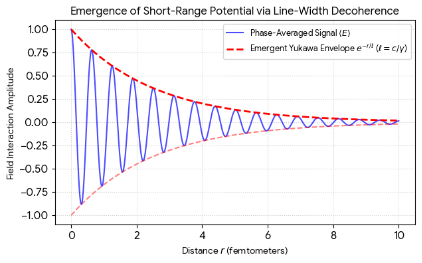
As an exclusive bonus for the blog—and a showcase of what even a free-tier AI model can produce when pushed by the right driver—Gemini generated a beautiful visualization of this exact phase-averaging phenomenon.
Below, we first produce the visualization in plain ASCII text, and then in a even nicer Python-genererated image. Both diagrams showcase how the high-frequency internal Zitterbewegung carrier wave naturally gives way to the macroscopic, short-range Yukawa envelope purely due to structural phase cancellation over distance:
The code can be visualized otherwise (see Python-rendering below) but it models the same thing: how a high-frequency Zitterbewegung oscillation, when subjected to a minor structural line-width frequency variation, naturally collapses into a clean, macroscopic Yukawa exponential envelope as distance r increases.
Such visual proofs-of-concept complement the math of our paper: they show that you do not need to invent an exchange boson. The finite geometry of the source acts as a natural spatial phase filter.
A Final Thought on Intellectual Honesty
I have explicitly credited the AI-assisted review both in my paper’s appendix and bylines as well as in this blog post itself. Some might wonder if using an AI this deeply is “cheating.” I don’t think so. The ontological architecture—the insistence on realism, spatial geometry, and anti-mysticism—is entirely human. The AI merely acted as a high-speed translator, digging through centuries of classical electrodynamics to find the precise mathematical analogies I needed.
If 64% of us are looking for a better interpretation of physical reality, we shouldn’t shy away from using every tool at our disposal to build it. Sometimes, a profound conceptual revolution begins exactly where standard calculation stops being satisfying—and a Saturday night wrestling match with a machine is a small price to pay for a clearer picture of the universe.
What struck me was not so much which interpretation came out on top, but rather the absence of any overwhelming consensus at all.
This is remarkable when one thinks about it. Quantum mechanics is, without doubt, the most successful physical theory ever developed in terms of predictive power. The equations work. Spectacularly well. And yet, almost a century after the Solvay Conferences, physicists remain deeply divided on what these equations actually mean.
That distinction matters: The mathematics is not in crisis but the ontology still is.
Let us, before proceeding to a deeper analysis, reproduce the exact survey question, the wording used to describe the Copenhagen interpretation, and the surprisingly fragmented result.
The survey asked: “Quantum mechanics can provide exceptionally accurate predictions of real-world phenomena. Yet, physicists cannot explain how the reality we experience emerges from the laws of quantum mechanics—a question that many ‘interpretations’ of quantum mechanics attempt to solve. In your opinion, which interpretation of quantum mechanics is most likely to be correct?”
The Copenhagen interpretation itself was described as: “an object’s behavior is described by a multi-state wavefunction, which collapses to one state when an object is measured.”
That description strikes me as reasonably accurate and fair. This makes the result even more surprising:
Only about 36% of respondents selected Copenhagen as the most likely interpretation. In other words, the so-called “mainstream” interpretation of quantum mechanics does not command anything close to a majority among the respondents to this survey.
This raises the question: why would we even call it “mainstream”?
Why is there no majority interpretation?
The answer is probably sociological rather than scientific. Copenhagen became the historical teaching framework of twentieth-century quantum mechanics. It became institutionalized. Textbooks adopted its language. Generations of physicists learned to “shut up and calculate,” often without worrying too much about the philosophical implications.
However, I think the survey also reveals something deeper: there remains substantial discomfort with the idea that the wavefunction is merely a probabilistic object with no deeper physical meaning:
Others embrace QBism, which interprets the wavefunction as an observer’s personal expectation rather than an objective feature of reality.
And then there is a surprisingly large “none of the above” category. I would definitely have chosen that option myself.
Why none of the above?
My own view does not align comfortably with any of the standard categories. In a broad sense, my interpretation may look somewhat like a hidden-variable approach. However, the term “hidden variable” is often misleading because it suggests adding extra variables to the formalism in order to restore determinism.
That is not really what interests me. What interests me is the possibility that some of the quantities already present in quantum mechanics — especially phase — may correspond to physically real processes rather than abstract mathematical bookkeeping devices. More specifically, I tend to think of the phase of the wavefunction as the phase of a real underlying oscillation:
The problem is not necessarily that reality is undefined.
The problem may simply be that the oscillation is too fast, too small, or too deeply embedded in the structure of matter for us to access directly.
In that sense, uncertainty may be operational rather than ontological. This is one reason why I continue to find Schrödinger’s old Zitterbewegung idea fascinating.
Dirac’s remarkable remark
Paul Dirac, in his 1933 Nobel Lecture, referred explicitly to Schrödinger’s interpretation of the electron as involving an extremely rapid oscillatory motion:
“This is a prediction which cannot be directly verified by experiment, since the frequency of the oscillatory motion is so high and its amplitude is so small. But one must believe in this consequence of the theory, since other consequences of the theory which are inseparably bound up with this one, such as the law of scattering of light by an electron, are confirmed by experiment.”
I find this quote extraordinary. Not because Dirac claims the oscillation was experimentally verified — it was not — but because he explicitly argues that one should still take the consequence seriously because the broader structure of the theory works so well.
That is a very different philosophical stance from modern textbook Copenhagenism, which often treats such internal structure as either meaningless or inaccessible in principle. Dirac’s remark effectively suggests that the oscillation might be physically real, even if it is experimentally inaccessible at present.
Phase realism versus probabilistic ontology
The modern interpretations debate often feels strangely constrained to me.
One camp argues that the wavefunction is merely information.
Another argues that all branches of the wavefunction are physically real.
Another introduces pilot waves.
Another introduces collapse processes.
But all of these approaches still inherit the standard ontology of the formalism more or less intact. My own discomfort lies, therefore, elsewhere.
I increasingly suspect that the equations themselves may be describing emergent phase-coherent behavior of deeper oscillatory structures rather than probability clouds existing in abstract Hilbert space.
That may sound radical at first glance, but it is actually rather conservative in spirit:
keep the equations,
keep the experimental predictions,
but reconsider what the variables physically represent.
the experimentally observed interference behavior may correspond to envelope or translational phase coherence,
while a deeper internal oscillatory dynamics remains hidden beneath the observable layer.
This is not an attack on quantum mechanics. Quite the opposite. It is an attempt to take some parts of quantum mechanics more literally than modern orthodoxy usually allows.
Final thought
The survey reminded me of something important. Despite the immense success of quantum mechanics, physics may still be in a strangely transitional period conceptually. The equations work. But the underlying picture of reality remains unsettled.
For decades, physics culture has often leaned toward the pragmatic “shut up and calculate” attitude: use the formalism, trust the predictions, and avoid asking too many questions about what the equations might actually represent physically. That attitude was understandable. Quantum mechanics works extraordinarily well. But surveys like this suggest that, beneath the practical success of the formalism, there remains no genuine consensus about the ontology underneath it. The equations may be spectacularly successful while our interpretation of their physical meaning remains incomplete.
Perhaps that is not a weakness of physics, but a reminder that some conceptual revolutions begin precisely where calculation alone stops being intellectually satisfying. After all, the history of physics itself shows that renewal usually begins not when equations fail, but when people start asking what the equations are actually trying to tell us.
The MIT press release was, unsurprisingly, ambitious: quantum weirdness may not require quantum mechanics after all. Classical physics, suitably reformulated, might already contain the essence of quantum behavior.
Hossenfelder’s response was sharp—and skeptical. In the video, she argues that the paper likely overstates its claims and may even contain a circular mathematical argument. More amusingly still, she notes that ChatGPT, Claude, and Grok all apparently agreed with her assessment almost instantly.
That, in itself, struck me as fascinating. So I did what one now apparently does in 2026: I asked “my” ChatGPT (by which I simply mean the instance shaped by years of my own ongoing projects, discussions and questions) what it thought about ‘her’ ChatGPT agreeing with her criticism of MIT physicists. The result was unexpectedly nuanced.
The AI largely agreed with Hossenfelder that the MIT press release probably exaggerates the implications of the work. Reformulating quantum mechanics using Hamilton–Jacobi theory, least-action principles, path integrals, or hydrodynamic analogies is not entirely new. Such bridges between classical and quantum formalisms have existed in various forms for decades.
At the same time, the AI also suggested that dismissing the work too quickly may itself miss the point. Reformulations can still be useful even when they do not overturn existing theory. Physics progresses not only through new equations, but also through new representations, computational shortcuts, and conceptual bridges.
But perhaps the most interesting part of the exchange concerned the role of AI itself:
Large language models are excellent at recognizing patterns, hidden assumptions, familiar forms of circular reasoning, and inconsistencies in argumentation.
But they are not theorem provers. Nor are they independent judges of truth.
They are strongly influenced by framing and context. In other words: if one asks skeptically, they often respond skeptically.
That realization feels oddly important. We are entering a moment in which AI systems are increasingly being invoked rhetorically in scientific discussions:
“ChatGPT agrees with me.”
“Claude confirms the derivation is wrong.”
“Grok spotted the flaw instantly.”
Perhaps useful. Certainly interesting. But not equivalent to mathematical proof.
For me personally, the discussion also clarified something else: I do not see this MIT work as confirmation of the sort of speculative ‘RealQM’ or particle-ontology ideas I have occasionally explored over the years on this blog and in open research fora such as ResearchGate or viXra.org.
The MIT approach remains fundamentally mathematical and formal: a reformulation of existing quantum mechanics. The questions that continue to interest me are rather different:
What is a particle, physically?
Does phase correspond to something physically real?
Is there a deeper internal structure or dynamics beneath the formalism?
Are some of the abstractions of modern quantum field theory descriptions of reality—or merely successful calculational tools?
Those are ontological questions more than computational ones. In that sense, this recent discussion also reminded me of a thought I had while reading Sabine Hossenfelder’s Lost in Math earlier this year.
Her critique of modern theoretical physics is often presented as deeply anti-mainstream—and in sociological terms, perhaps it is. She sharply criticizes the overreliance on beauty, elegance, symmetry, and speculative mathematical aesthetics. I largely agree with that critique.
But I increasingly suspect that her criticism still operates largely within the conceptual boundaries of the Standard Model and contemporary quantum field theory. The mathematical formalism itself is rarely questioned at the level of physical interpretation.
My own dissatisfaction lies elsewhere. Not with mathematics as such, but with the possibility that modern physics may sometimes confuse predictive success with genuine understanding. Or, as I wrote in an earlier post inspired by Lost in Math:
“The real challenge is not to extend the mathematical formalism, but to understand what the existing formalism is telling us about physical reality.”
Looking back, this also feels like an appropriate reflection for what happens to be the 400th post on this blog since I started writing Reading Feynman in 2013.
Over time, the project gradually evolved away from the excitement of speculative “breakthroughs” and toward something quieter: trying to reduce the sense of mystery surrounding quantum mechanics without pretending to have “solved” it.
Not by rejecting mathematics, but by repeatedly asking what the mathematics is actually saying.
Not by dismissing mainstream physics, but by trying to distinguish between prediction, interpretation, ontology, and scientific storytelling.
And perhaps also by becoming increasingly skeptical of hype in all its forms:
hype surrounding speculative theories,
hype surrounding anti-hype,
and now perhaps even hype surrounding AI-assisted certainty itself.
Modern science communication sometimes oscillates between simplification and debunking, with each side occasionally amplifying the other. Meanwhile, quantum mechanics remains quantum mechanics. And perhaps that is why I found this whole MIT / Hossenfelder / AI-discussing-AI episode so strangely revealing:
The MIT press office oversimplifies.
The YouTube critique oversimplifies the oversimplification.
AI systems then participate in evaluating the critique of the oversimplification.
Interesting times.
PS: One unexpected consequence of this whole “humans versus AI” controversy is that it pushed me — with, yes, AI itself — to think much more deeply about statistics, ontology, prediction, meaning and intelligence. The result is this new paper: “Quantum Statistics and Ontological Modesty: Reconsidering the One-Slit Problem”
The paper revisits Feynman’s famous lecture on quantum behavior, questions whether statistical success necessarily implies ontological randomness, and explores parallels between quantum interpretation and modern AI systems.
For those interested in pushing the boundaries of both human and artificial intelligence — philosophically rather than ideologically — the paper may be worth a read. 🙂
For quite some time, I have been trying to understand elementary particles—especially the electron—as structured objects rather than point-like entities. The intuition was simple: instead of something static, imagine something that moves, something that circulates.
In earlier work, I explored models in which charge moves in a loop—what you might call a ring current. That idea turns out to be surprisingly powerful. It naturally connects to the electron’s magnetic moment, its angular momentum, and even to a characteristic length scale that seems to “fit” remarkably well with what we know from quantum physics.
So at first sight, it feels like you’re onto something.
But then the cracks start to appear.
The first issue is familiar: a charge moving in a circle should radiate. That alone already makes the picture problematic. But even if you try to work around that, deeper questions arise. What is actually holding this motion together? What is acting on what? And—more fundamentally—what does it even mean to speak of a “charge” moving at that scale?
At some point, I realized that the problem might not be the idea of circulation itself, but what is assumed to be circulating.
Instead of imagining a charge moving along a trajectory, I now look at the possibility that what circulates is not charge, but energy. In that picture, the electron is no longer a particle following a path, but a localized configuration of fields in which energy continuously flows in closed loops.
This change sounds small, but it turns out to be conceptually important. It removes the need to talk about a point-like object moving at extreme speeds, and replaces it with a structure that is, in a sense, stationary—even though internally something is still “going round and round.”
Interestingly, this field-based picture manages to preserve much of the original intuition. You still get circulation. You still get angular momentum. You still get a natural scale that ties energy to motion. In that sense, the original idea wasn’t wrong—it was just expressed in a way that leads to inconsistencies.
However, the new formulation also makes something else very clear.
Electromagnetism alone is not enough.
If you analyze the balance of forces in such a configuration, you find that things almost work. Electric and magnetic effects can nearly compensate each other. There is a kind of near-equilibrium that reflects the original intuition of something “held together” dynamically.
But “almost” is not good enough.
There is no true stability. No mechanism that fixes the size of the structure. No reason why it should not simply expand or dissolve.
That turns out to be the key insight of the paper, which you can find here.
If we want a stable, particle-like object, something else must be present—some additional ingredient that provides a form of tension or confinement. In the paper, I explore a couple of simple toy models that illustrate how such stabilization might arise. They are not meant as final answers, but as minimal examples of what is required.
So where does that leave the original idea?
Not discarded—but refined.
The notion that particles are built from circulating something still seems meaningful. But it is no longer “charge moving in space.” It is better understood as energy organized into a persistent pattern—a structure that maintains itself through the interplay of fields and whatever additional mechanisms are needed to stabilize it.
This paper is part of an ongoing attempt—what I’ve loosely called the “RealQM” approach—to explore how far such intuitive, semi-classical ideas can be pushed, and where they inevitably run into the need for a deeper framework.
It does not offer a finished theory. If anything, it does the opposite: it makes very clear where the simple models break, and why.
But that, too, is a form of progress.
Post scriptum (May 2026) — Since writing this post, I have published a companion piece:
While the earlier paper focused on the limitations of purely electromagnetic models (and the need for some form of stabilizing structure), this follow-up takes a step back and asks a broader question:
Why do the same mathematical structures keep appearing across different areas of physics?
In particular, it explores how:
a simple stability condition leads to a preferred length scale,
that structure naturally becomes “quadratic” near equilibrium,
and how this connects directly to the harmonic oscillator and the appearance of discrete energy levels (as discussed by Feynman).
The paper is not especially technical. Its aim is to connect the mathematics to physical intuition, and to show how ideas that often appear abstract—like oscillators, eigenvalues, or quantization—can be understood as different aspects of the same underlying structure.
If you’ve ever wondered why the math in quantum mechanics looks the way it does (rather than just how to use it), you may find this piece a useful complement to the discussion here.
I finally got around to reading Sabine Hossenfelder’s ‘Lost in Math‘ (2018).
It fully deserves its praise. The book is, as the reviewers write, accessible, well-informed, and engaging—at times even genuinely funny. The structure, built around interviews with leading theorists, gives it both breadth and credibility. It is, without doubt, one of the better popular accounts of modern theoretical physics.
It also felt familiar.
Hossenfelder and I belong to roughly the same generation. As teenagers in the 1980s, we were fascinated by the same questions: What is the Standard Model really about? Where did it come from? What problems did it solve that even Albert Einstein or Max Planck could not? And what new questions did it open?
And then, of course, the next layer: why do we need theories beyond it—string theory, supersymmetry—if the Standard Model already works so well? What are these theories trying to explain that the Standard Model cannot?
And what should we make of the experimental side of things? From the discovery of the Higgs boson to the evidence for dark matter, dark energy, and gravitational waves—what do these findings actually mean?
Hossenfelder chose to pursue these questions within academic physics. I did not. I studied economics, but continued to explore physics as a personal project—especially after 2012, when the Higgs boson was announced. By then, I had grown dissatisfied with popular science accounts and felt the need to understand the mathematics itself.
And yet, after working through the math, I found myself asking a different kind of question: not whether the equations work, but what they mean.
It is here that Hossenfelder’s book, for me, remains incomplete.
Beauty, Truth—and Something Missing
The central argument of Lost in Math is well known: modern theoretical physics has been led astray by an overreliance on aesthetic criteria—symmetry, elegance, mathematical beauty—at the expense of empirical grounding.
That critique is compelling, and I largely agree with it.
But it seems to stop halfway.
While Hossenfelder questions the role of beauty, she does not fundamentally question the underlying framework itself. The Standard Model and its extensions remain, in her account, the unquestioned language in which physical truth must ultimately be expressed.
What is largely absent is a deeper discussion of physical interpretation.
The Question of Meaning
Let me be more concrete.
The book does not attempt to explain why the strong force could not be understood in more classical terms, for example as some form of electromagnetic interaction arising from internal charge dynamics.
It does not address why abstract quantum numbers—color charge, flavour, isospin—should be regarded as physically compelling, rather than as mathematical constructs that work but lack intuitive grounding.
Likewise, the weak force appears mainly as part of a formal structure, without much discussion of what it might represent in more tangible terms—such as the distinction between stable and unstable particles.
And perhaps most strikingly, the book does not engage in any depth with the meaning of the most fundamental relations in physics: the quantization expressed in the Planck relation, or the significance of mass-energy equivalence. These are presented as known facts, not as conceptual puzzles.
None of this is a flaw in the usual sense. It is simply not the book Hossenfelder set out to write.
But it is the book I was hoping to read.
Old Physics, Reconsidered
So where does that leave us?
In my own work, I often find myself returning to what many would call “old physics”: Maxwell’s equations, together with relations like Planck–Einstein relation and mass–energy equivalence.
This may seem old-fashioned. Perhaps it is.
But I am increasingly convinced that the real challenge is not to extend the mathematical formalism, but to understand what the existing formalism is telling us about physical reality.
From that perspective, the problem is not only that modern physics may have followed beauty too far. It is also that it may have drifted too far from meaning.
A Different Kind of Dissatisfaction
Hossenfelder ends her book on a note of optimism. Physics, she argues, will continue to make breakthroughs, and those breakthroughs will—once again—be beautiful.
I hope she is right.
But closing the book, I was left with a different thought. Not frustration, but a kind of clarity.
I realized that I am quite content continuing to explore these questions from a more classical, more intuitive starting point—even if that places me outside the mainstream.
Because, in the end, the question that still matters most to me is a simple one:
Not whether the mathematics works, but whether we truly understand what it is saying.
Post scriptum on the 2019 revision of SI units
Sabine Hossenfelder finished and published her book in 2018—just before the 2019 revision of the SI units.
I find myself wondering whether that revision is, in its own quiet way, more meaningful than many of the theoretical developments discussed in her book. Perhaps I am over-interpreting, but this is how it looks to me.
The revised SI system fixes exact numerical values for a small number of fundamental constants, such as the Planck constant, the elementary charge, and the speed of light. In doing so, it anchors our system of measurement in quantities that are directly tied to observation and experiment.
What is striking, however, is what it does not include.
There is no place in the SI framework for the various additional “charges” or quantum numbers that appear in the Standard Model—no color charge, no flavour, no isospin. These concepts may be essential within the mathematical structure of modern particle physics, but they do not enter the system that defines how we measure physical reality.
This is not a flaw in the SI system—quite the contrary. It is designed to remain independent of theoretical interpretation, and to rely only on quantities that can be operationally defined and reproducibly measured.
But that, in itself, is revealing.
It suggests a distinction between what we can measure directly and what we introduce as part of a theoretical framework. And it raises a question—at least for me—about how closely our most advanced theories are tied to physically meaningful quantities.
None of this diminishes the achievements recognized by a Nobel Prize in Physics or other honours—or the remarkable success of modern theoretical physics more generally. But it does serve as a quiet reminder that predictive success is not the same as final understanding.
If anything, the SI revision reinforces my own inclination to look for interpretations of physics that remain as close as possible to what can be directly measured and understood.
Post-Post-Scriptum on what I would like to write
Since writing this, I’ve taken a small but meaningful step: I uploaded a somewhat older manuscript and a newly written Chapter 2 to ResearchGate, as companion documents to my Radial Genesis paper (thoughts on cosmology).
It is not as a finished book — far from it — but as a snapshot of where my thinking currently stands. If I were to write a full-blown book about this, it would not be a technical monograph, nor a speculative manifesto. It would be something in between: a guided journey. I would try to connect three layers:
the physical intuition (what kind of universe are we actually living in?),
the mathematical structure (how symmetry, geometry, and scaling laws shape that intuition),
and the cosmological narrative (how a finite universe with emergent spacetime could naturally arise).
Most importantly, I would try to bridge particle physics and cosmology — not as separate domains, but as different perspectives on the same underlying structure.
The current documents are fragments of that attempt. For now, I will leave them as they are. Sometimes it is better to pause, let ideas settle, and return later with fresh eyes.
Post-post-post-scriptum
I couldn’t help thinking about this question: if the math in academic physics has become “ugly” or “lost,” then what would a beautiful alternative look like? Of course, ‘beauty’ (for me, at least) is a combination of simplicity and realism, and so that is my ‘RealQM’ world view. So I did a quick paper on ResearchGate on what Sabine Hossenfelder still thinks of as very ‘mysterious’ but which, to me, is easily explained in my ‘RealQM’ framework’:
The “Ghost” Sector (Dark Matter): Two types of electromagnetism (defined by the fundamental asymmetry in Maxwell’s equations modern mainstream physicists completely ignore) share the same spacetime but do not interact otherwise. Because they share the same spacetime, they do interact ‘gravitationally’. Full stop: no further explanation needed.
The Proton Radius: My two-line theoretical calculation gives a proton radius of 0.841 fm. Recent measurements clocked the proton at 0.8406(15) fm. What more confirmation is needed to urge physicists to think of particles as dynamical structures rather than abstract entities with lots of abstract or non-measurable properties?
Needless to say: challenges are still out there, and AI baptizes one of them now officially as The Geometry Challenge or Proton Yarnball Puzzle.
The X-lectures series complement our previous Lectures series on ResearchGate on electromagnetic and quantum theory from a classical perspective, which we define as making sense of Maxwell’s equations and the Planck–Einstein relation from what we call a realist perspective. The objective of this new series is not to oppose modern physics, but to better understand it—by carefully revisiting some of its foundational assumptions.
The starting point is Lecture X1, in which we operationalize the distinction between stability and instability of charged particles through a simple but physically meaningful quantity: the phase-closure defect . Instead of treating decay as fundamentally probabilistic, we interpret it as the gradual loss of phase coherence in an internal dynamical structure. This provides a concrete example of what we call a statistical determinist reading of quantum phenomena.
Lecture X2 then revisits the concept of a gauge in classical electromagnetic theory. While gauge freedom is usually presented as a harmless mathematical redundancy, we argue that it is not entirely “innocent”: the choice of gauge reflects boundary conditions, physical assumptions, and the way we organize the description of interactions.
In Lecture X3, we take a further step. Modern physics elevates gauge symmetry from a freedom of description to a guiding principle from which interactions are derived. We examine this move carefully and contrast it with a realist interpretation in which the phase of the wavefunction represents physical structure rather than a purely mathematical degree of freedom. From this perspective, gauge fields may be seen as arising from consistency requirements of the formalism, rather than as fundamental entities.
Taken together, the three papers trace a conceptual progression:
from stability as phase coherence (X1)
to gauge freedom as non-trivial choice (X2)
to gauge principles as powerful—but possibly non-fundamental—structures (X3)
In essence, we move from a “gauge is not innocent” position to a “gauge may not be fundamental” position.
The broader aim is modest but, we think, important: to show that the standard formalism of modern physics remains operationally complete, while its interpretation is not unique. Exploring alternative ontologies—such as the realist perspective adopted here—may help clarify what our equations are actually telling us about physical reality.
Links to the papers (X1: Operationalizing the Stability–Instability Frontier, X2: Intuitive Notions on Gauge Theory, X3 From Gauge Freedom to Gauge Principles—and Beyond) are in the text above.
As always, comments are welcome—but preferably in the form of arguments, equations, or better ideas.
Every student of physics encounters the so-called classical electron radius. It is usually introduced as a curious length scale that appears when one equates the rest energy of the electron with the energy stored in its electrostatic field.
The reasoning is simple enough. If the electron’s charge were somehow concentrated within a sphere of radius r, one can calculate the energy stored in the electric field surrounding that charge. Setting that field energy equal to the famous E = mc² gives a radius of about 2.8 femtometer.
This number has been known for more than a century and is still quoted in textbooks. Yet its physical meaning has always been somewhat puzzling. The derivation relies on a rather arbitrary assumption: that the electron’s rest energy originates entirely from its electrostatic field.
In a recent paper I revisited this question from a different angle. Instead of thinking of the electron as a static charged sphere, one may think of it as having a dynamical structure: a circulating charge. Such a motion – just the good old magnetic or ring current model of an electron – naturally produces a magnetic moment, and when one calculates the radius required to reproduce the observed magnetic moment of the electron, a very familiar scale emerges: the Compton radius.
This leads to a simple hierarchy of length scales:
Compton scale (internal dynamics) ↓ Classical electron radius (re = a·rC) ↓ Coulomb field extending outward to infinity
In other words, the classical electron radius does not represent the literal size of the electron. Rather, it appears to be the electromagnetic coupling scale associated with a charge circulating at the Compton radius.
From this perspective the rest energy of the electron is not stored in its external Coulomb field. Instead, it may be associated with the internal electromagnetic dynamics of the circulating charge. The familiar Coulomb field is then simply the long-range electromagnetic “tail” of that dynamical structure.
Looking at the problem in this way also suggests a natural question about the proton. If one performs the same classical self-energy calculation for the proton, one obtains a radius far smaller than the experimentally measured proton radius—by roughly a factor of five hundred. This striking difference hints that the electron and the proton, although carrying the same unit charge, may correspond to very different internal charge dynamics. To be precise, we think of the proton as a three-dimensional oscillation of charge (as opposed to the two-dimensional ring current model for the electron).
Another numerical curiosity emerges in this comparison. Physicists often marvel at the small value of the fine-structure constant (see our previous post on that). Yet the much larger ratio between the proton and electron masses—about 1836—may be even more mysterious. Two particles carrying identical charge nevertheless differ enormously in mass and characteristic size.
Perhaps the most important lesson of all this is methodological. The classical electron radius should probably not be interpreted as the size of the electron. It is better understood as a scale that reflects how strongly the electron couples to the electromagnetic field.
Seen in this light, the old “classical” radius acquires a new and rather natural meaning within a dynamical electromagnetic picture of the electron.
Over the years I wrote several short papers and lecture notes touching on the fine-structure constant (α ≈ 1/137). Some of these appeared on viXra, others were used as slides for YouTube lectures, and still others were scattered across different notes and working papers on my ResearchGate page.
I recently decided it was time to bring those ideas together into a single, more coherent manuscript. The result is a new preprint — Revisiting the Meaning of the Fine-Structure Constant — which I have now uploaded on ResearchGate. The earlier slides remain available as supplementary material.
The motivation for the paper is simple. In popular physics, the fine-structure constant is often presented as a mysterious number. Richard Feynman famously asked why the universe “chooses” a value close to 1/137. Instead of treating α as a mystery, the paper asks a more basic question: what physical quantities does this dimensionless ratio actually compare?
Seen from that perspective, several familiar appearances of α fall into place.
First, the constant emerges as a geometric scaling ratio between characteristic electron length scales, linking the classical electron radius, the Compton radius, and the Bohr radius in a simple ladder.
Second, the constant can be interpreted as a ratio of energy–length scales, comparing the strength of the electromagnetic interaction (through the Coulomb factor) with the quantum-relativistic action scale (which combines Planck’s quantum of action h and lightspeed).
The paper also revisits the appearance of α in the hydrogen spectrum and, yes, also briefly discusses its role as the electromagnetic coupling constant in quantum electrodynamics (QED). In fact, the latter addition is an unusually sympathetic look at the modern perturbative approach that is so common in modern quantum field theory: we acknowledge we used AI to make sure it would not sound too biased. 🙂
In any case: taken together, these perspectives suggest that the fine-structure constant is less mysterious than often suggested. Rather than being an inexplicable number, it acts as a compact bridge linking classical electromagnetism, quantum theory, and atomic structure.
Every student of physics learns that the magnetic moment of the electron is given, to first approximation, by what is referred to as the Dirac value or – the more commonly used term – the Bohr magneton:
μe = μB = (ħ/2)·(qe/me)
We separate the two factors in it because our (neo-classical) RealQM framework interprets (i) the qe/me factor as a form factor which distinguishes the electron from, say, a proton or the more massive muon-electron (how much charge per mass or energy unit is ‘packed’ into the particle?), and (ii) ħ as the ubiquitous quantum of action that determines how energy, linear or angular momentum, or – in this case – magnetic moments are quantized. Think of it like this: charge comes in lumps (elementary charged particles), and its dynamical properties come in lumps too.
What about the 1/2 factor? We must refer to our Lecture on Quantum Behaviorhere for a rather common-sense interpretation of the g-factor and the spin-1/2 property of elementary matter-particles. The electron – interpreted as a dynamic oscillation of charge – ‘packs’ one Planck unit of physical action in each cycle of the oscillation but the angular momentum of the orbiting charge only explains half of the energy (and, therefore, the mass of the electron). The other half is in the electromagnetic field it generates, which keeps the charge spinning and effectively explains the magnetic dipole moment. So, just like protons or the more massive muon-electron, the electron can effectively be described as a ‘fermionic’ or ‘spin-1/2’ particle.
So far, so good. Experiments, however, show that the actual (measured) value is slightly larger. The difference is tiny—about one part in a thousand—and is known as the anomaly in the magnetic moment.
Modern physics explains this anomaly through quantum electrodynamics (QED). In that framework, the correction arises from increasingly complicated perturbative calculations involving “loop diagrams.” The first term in the resulting expansion was derived by Julian Schwinger in 1948 and is equal to /2. That is a very elegant expression, and it explains the anomaly for about 100.15%. Two quick notes must be made here:
1. We effectively wrote: 100.15%. Not 99.85%. Why? Because Schwinger’s factor overshoots the anomaly effectively by about 0.15%. To be precise, (μCODATA-μe)/μe = 0.00115965… and CODATA/2 = 0.0011614… The fact that the Schwinger term slightly overshoots the experimentally measured anomaly, explains why the next correction in QED is actually negative: it must bring the theoretical prediction back into agreement with experiment. This sign swap is rather poorly explained in standard textbooks but, in any case, it is any classical or neo-classical interpretation must probably reproduce such sign patterns. However, in our paper – which is just an introduction to our thinking on this – we do not go into that: we basically just explain – using classical arguments – why α and 2 appear so naturally not only in the leading correction but also higher-order corrections to the Dirac value for the electron’s magnetic moment.
2. Note that we take CODATA values here because these reflect (i) the scientific/academic consensus on the measured magnetic moment (as opposed to the theoretical Dirac value) and (ii) the scientific/academic consensus on the value of the fine-structure constant. The 2019 revision of the system of SI units effectively adds an interesting twist to the debate: the fine-structure constant itself is now defined as being co-determined with the electric and magnetic constant, and the standard relative uncertainty of all three constants is, therefore, now exactly the same: 1.610-10, to be precise.
Let us now go back to the main story line. From the above, it is clear that, while the precision of Schwinger’s factor is higher than 0.15% of one part in a thousand (so that’s a precision of 1.5 parts into a million), we still need higher-order corrections. Why? Because measurements are much more accurate than one part into a million, and some theory should explain all significant digits, isn’t it? 🙂
Using the QED/QFT framework, theoretical physicists have currently computed those higher-order corrections up to what is referred to as the ‘five-loop level’ in QED, with astonishing agreement between theory and experiment. The problem with this ‘astonishing agreement’ is its complexity: the calculations become evermore complicated – as evermore degrees of freedom (cf. the increasing number of Feynman diagrams, which illustrate the various ways in which something might happen) explain less and less, as illustrated in the table below.
In a recently revised working paper on ResearchGate, I therefore explore a different question. Instead of asking how the anomaly emerges from perturbative quantum field theory, I ask whether the structure of the leading correction might also admit a classical interpretation. In the next section, we explain the basics of this classical interpretation, which is based on the ring current model of an electron, which was first advanced by Alfred Lauck Parson in 1915 and, as we explain in our paper on the nature of de Broglie’s matter-wave, also naturally explains Schrödinger’s Zitterbewegung theory. In other words, it is a very classical approach. 🙂
The electron ring current model
The starting point is, effectively, the old ring-current picture of the electron: imagine a localized “blob” of charge circulating around some center at the speed of light. This blob of charge has no other properties (no rest mass or rest energy) but its charge and, yes, some non-finite size. To be precise, from scattering experiments and the formulas that describe photon-electron scattering, we assume its size is of the order of the classical electron radius. As for the assumption of lightspeed, it is only logical to assume that anything with zero rest mass must travel at lightspeed because the slightest force on it will accelerate it to lightspeed.
When we apply this idea to the electron charge, we must conclude that the radius of this orbital motion will be the Compton radius of the electron. Indeed, when we think of the (elementary) wavefunction r = ψ = a·eiθ as representing the physical position of a pointlike elementary charge – pointlike but notdimensionless – moving at the speed of light around the center of its motion in a space, we must conclude that the radius of this orbital motion – which effectively doubles up as the amplitude of the wavefunction – must be equal to the electron’s Compton radiusa = ħ/mc. This can easily be derived from (i) Einstein’s mass-energy equivalence relation, (ii) the Planck-Einstein relation, and (iii) the formula for a tangential velocity:
This electron model also naturally yields the Dirac magnetic moment: we can just calculate it using the standard formula for the magnetic moment of a ring current.
The next step, then, is to acknowledge that charge cannot literally be pointlike. If the circulating charge has a finite spatial extent—of order the classical electron radius—then the current distribution is slightly modified. The mathematical and physical elegance of Schwinger’s factor can then easily be explained by:
(i) noting that the classical electron radius is times the Compton radius of the electron ħ/mec = ħc/Ee, which – in all mainstream accounts of photon-electron scattering experiments – is the scale at which the (free) electron can be localized in a particle-like sense (for more precise academic references (we like LeClair’s (2019) straightforward derivation and textbook explanation of Compton scattering), see our paper on de Broglie’s matter-wave); and
(ii) noting that the 2 factor points at orbital rather than linear motion. Indeed, a division by 2 is all what we need to do whenever we want to relate an orbital velocity or length (a linear wavelength or, when orbital motion rather than linear motion is involved, which is the case here) to radians rather than the SI unit for distance. More generally speaking, the factor pops up whenever we evaluate some loop integral (i.e, whenever we integrate some quantity over a closed orbit using the phase of the (orbital) oscillation).
This strongly suggests that – from the various physical relations in which the fine-structure constant pops up – we should explore its meaning as a scaling constant. More in particular, the fine-structure constant here is the ratio which relates the classical electron radius and the Compton radius. We do not want to distract the reader too much but it is probably good to immediately point out that this interpretation of the fine-structure constant as a geometric ratio is also valid when examining the relation between the Compton radius (free electron) and the Bohr radius (the radius of the negative charge as it manifest itself in a hydrogen atom):
re = α·rC ( 2.81810-15 m), rB = rC/α ( 0.52910-10 m), and rC = ħ/mec = = ħc/Ee ( 386.5310-15 m)
This is intriguing because it shows a 1: 1/α : 1/α2 ‘ladder’ or ‘series’ for the value of (i) what we think of the radius of the elementary charge, (ii) the radius of the elementary particle (free electron) in which this charge manifests itself, and (iii) the interaction radius of the bound electron in its most basic state (i.e., bound by a proton in the hydrogen atom). Needless to say, the multitude of physical phenomena in which the fine-structure constant pops up clearly illustrates that measuring its value can be done in a variety of ways. Measuring it through ever more precise measurements of the anomalous magnetic moment is, therefore, just one way to go about it.
To sum it all up, the hypothesis of a pointlike charge with radius re = α·rC is in completely alignment with the suggestion that (i) any first-order correction to the ideal ring current must scale with α and (ii) because the circulating motion is periodic, any cycle-averaged correction would naturally come with a ‘normalization’ over the full () phase of the orbit. Put these ingredients together and one obtains a leading correction with the same structure as Schwinger’s factor:
Δμ/μe ≈ /2
This does not necessarily replace the first-order QED derivation – especially because we should note that first-order QED calculations are based on the classical electromagnetic equations anyway – but it suggests that the form of the leading term may reflect a simple geometric fact: a finite electromagnetic structure (the ‘naked charge’ inside of a electron, as we call it) undergoing coherent circular motion.
The question, of course, then becomes: what about the higher-order corrections? What geometric or other common-sense arguments could one advance to explain second- or third-order scaling with α. In other words, why would terms with α2 or α3 – or, more generally, (/2)2n – pop up in any theoretical series of powers of α explaining the measured anomaly in the magnetic dipole moment of the electron?
That is what we are discussing in our paper, which we summarize and also comment on this blog post.
Again: why worry about an imprecision of about 1.5 parts in a million?
Again, the casual amateur physics may be tempted to let go of these discussions. The anomaly itself is tiny. The Dirac value already gets the magnetic moment right to about 0.1%, and the famous Schwinger correction then explains almost all of that 1% (about 100.15%, as we wrote). So, the higher-order QED terms only account for a very tiny fraction of the anomaly: something like 0.00015% (so that’s 1.5 parts in a million, indeed). So, why should we look for alternative or more comprehensive interpretations?
The answer is this: because the anomalous magnetic moment is one of the most precise measurements in all of science. Therefore, understanding why i) its leading structure has the form (/2 but (2) at the same time, why this leading structure does not fully explain the measured anomaly is not merely a numerical curiosity. It should tell us something about the underlying geometry of electromagnetic interactions. In other words, the tiny discrepancy carries a lot of conceptual weight.
This ‘conceptual weight’ may be illustrated by noting the complexities in QED/QFT calculations. They seem to contradict Occam’s Razor Principle: evermore complicated calculations – which result from allowing evermore degrees of freedom in the higher-order analysis, as illustrated in the table above – seem to explain less and less.
That is probably one of the reasons why there is discontent with the approach even in mainstream academics. We will let the reader google this – we warmly recommend Google’s Gemini assistant in this regard – but, as an example, it looks like lattice theory is currently rapidly emerging as a strong non-perturbative approach to ‘explaining’ the anomaly. [We put ‘explaining’ in brackets because, as far as we can see, lattice theory is, just like QED/QFT a predominantly mathematical approach, in the sense that its first principles are mathematical principles rather than physical laws). Below we briefly highlight this competing approach within the so-called Standard Model, which makes one wonder if there is still a thing such as a ‘standard’ model for explaining physics.
Perturbative QED: Treats interactions as small corrections (powers of the fine-structure constant) using Feynman diagrams. This works for the electron because its coupling is weak, but the complexity grows exponentially at higher orders.
Lattice Theory: Discretizes spacetime into a 4D grid (lattice) of points. It calculates interactions directly from first principles using Monte Carlo simulations on supercomputers, rather than summing infinite series of diagrams.
We must also note to another scientific breakthrough which, in our not-so-humble view, has received insufficient attention, and that is the 2019 revision of SI units. Let us discuss the most salient points of this very significant scientific revision.
The fine-structure constant and the 2019 revision of SI units
The extraordinary precision of the anomaly measurement is very closely connected to the discussion on (i) what the fine-structure constant α. actually is or represents in physics (as mentioned above, it pops up in many relations and equations) and, accordingly, (ii) how we should measure it.
Historically, α was measured through a variety of experiments and then used as an input for theoretical calculations. QED/QFT may be said to have inversed that logic: the measurement of the electron’s anomalous magnetic moment are used to then insert it the QED expansion, which is then used to solve for α. The result is, effectively, one of the most precise determinations of the fine-structure constant currently available but, to me, it looks like the 2019 revision of the SI system changed the conceptual landscape. Indeed, the 2019 revision of SI units clearly implies that (i) the fine-structure constant, (ii) the electric constant, and (iii) the magnetic constant must be co-determined because of the following physical equations:
Hence, the 2019 revision of SI units – which, we think, incorporates all of physics – makes it clear that, unlike precisely defined units such as the meter, second, charge, or exactly defined constants of Nature – such as the speed of light, charge, and the quantum of action – neither of these three constants of Nature (electric constant, magnetic constant, and fine-structure constant) have exact values: they must, effectively, be measured in physical experiments and, importantly, their values must be co-determined in such experiments. Indeed, the relations above imply that the relative standard uncertainty in the measures for all three constants, which is currently at 1.610-10, must remain the same in order to ensure conceptual agreement between experiment and theory.
We will not dwell too long on this because we ourselves still need to think through this some more. However, what we write above makes it obvious that this is very important when considering claims about the precision of both the experimental data as well as theoretical arguments on the anomaly: the precision is, indeed, extraordinary – and will probably become even more extraordinary over the coming decades – but, when evaluating any theoretical model explaining this anomaly, it is obvious such theory can no longer be viewed in isolation. Other physical interpretations of the fine-structure constant – such as the geometric interpretation we advance here – must also be considered.
Note: The above probably explains why CODATA remains rather conservative (as compared to the precision of experimental measurements, that is) in its consensus value for the fine-structure constant and the two electromagnetic constants: their value only has roughly ten significant digits. That is about 10000 times better than one part in a million but, still, it effectively does not quite reflect the accuracy of modern-day experiments. Instead, this standard relative uncertainty now probably reflects both theoretical as well as experimental uncertainties, and the theoretical uncertainties should, in our not-so-humble view, also include a critical analysis of the modern-day QED/QFT framework.
Classical or neo-classical explanations of higher-order terms
Again, the aim of our paper is not to fundamentally question or replace quantum electrodynamics, which seems to remain one of the most successful theories ever constructed. Rather, it is to ask whether the leading structure and higher-order corrections in the mainstream explanation of the anomalous magnetic moment might also admit a complementary geometric or other morefundamental interpretation. We think it does. Let us list all obvious elements of such more fundamental interpretation:
1. The Bohr magneton or Dirac’s formula for the magnetic dipole moment emerges naturally from the age-old electron ring current model, which was first advanced by Alfred Lauck Parson in 1915 and, as we explain in our paper on the nature of de Broglie’s matter-wave, also naturally explains Schrödinger’s Zitterbewegung theory.
2. The first-order correction (Schwinger’s factor) emerges, equally naturally, from the assumption that something that is infinitesimally small (i.e, something with zero physical size) does not exist and, hence, that (i) charge must have some size, and (ii) that, for an electron, this size is given by the classical electron radius. The inuuition here was explained above, and the detail of it is described in the paper we want to promote here. [You would not expect us to just copy-paste our paper in a blog article, isn’t it? :-)]
3. To explain the necessity and/or emergence of second- and higher-order terms, we think of the following:
(i) The assumption of an oscillation naked charge – whose size is not infinitesimally small but of the order of the classical electron radius – inside of the electron naturally leads to what we refer to as ‘finite-size’ corrections to the Compton radius. These corrections probably scale just like α but, when allowing for more advanced ideas such as self-interaction (we admit that we are not a fan but, when everything is said and done, self-interaction is an idea which the classical physicists did like to explore), may also be linear in α2, α3 or higher-order terms.
(ii) Intrinsic spin is, of course, a very obvious candidate for a correction of the core Dirac value of the magnetic moment of an electron. Indeed, if one thinks of the electron as an oscillation of some naked charge, then this small charge distribution itself should make one rotation around its own axis as it orbits around the center of the electron and, hence, this must result in a combined magnetic dipole moment that is slightly different from the Bohr magneton. We asked AI (ChatGPT) to do a quick calculation and – using the standard formula for the magnetic moment of a uniformly charged solid sphere of radius re rotating around its own axis with the same angular velocity ω as its orbital motion – the ratio of (1) this intrinsic magnetic moment and (2) the orbital magnetic moment (i.e., the Bohr magneton) should equal 4α2/5. In other words, this intrinsic spin effects enters at order α². Hence, this is structurally consistent with the observed perturbative hierarchy, in which the leading correction is proportional to α, and higher-order corrections scale with higher powers.
In our paper, we refer to the above alternative explanations as the ‘finite-size’ and ‘intrinsic dipole’ contributions to the magnetic moment, respectively, and we treat them in one and the same chapter because, as mentioned, they are prime candidates for the first- and second-order corrections to the theoretical magnetic moment of the electron.
As for higher-order corrections, we worked with AI to identify a number of additional candidate explanations. Frankly, these convince us somewhat less than the obvious theoretical remarks above but they cannot be dismissed out of hand. We, therefore, list and detail these in a separate chapter in the paper. They include explorations of:
(iii) The precessional motion ofthe presumed blob of charge in the electron, which one would expect it to have as a result of its intrinsic spin: such and like effects may also be referred to as projection effects resulting from the fact that, in real-life experiments, the free electron is being contained in a Penning trap by an electromagnetic field with which it obviously interacts. The measurement, therefore, must take into account various additional motions – such as complicated precessional or nutational motion – which, again, we will just categorize under the category of ‘projection effects’. [We recommend the reader to dive into the intricacies of what a Penning trap actually is, and look at the amazing technologies involved: a Penning trap combines (i) a homogeneous, strong axial magnetic field for radial confinement as well as (ii) an electrostatic quadrupole field to provide axial confinement.]
(iv) Various interactions which may be categorized as presumed classical ‘self-interaction’ effects. Such effects include interactions betweenpresumed charge elements within the blob, or between the blob and the electromagnetic field sustaining its motion. However, we intuitively feel one can think of many self-interaction effects and, therefore, these theoretical candidate contributions feel quite ad hoc.
(v) Finally, ChatGPT also alludes to complicated corrections that might or should be made as a result of the cycle-averaging or dynamical smearing which is inherent to the ring current model. Indeed, we treat a continuous current distribution just the same as a localized charge in some regular orbital motion. While one might argue we are looking at scales here at which Maxwell’s equations combined with the Planck-Einstein relation might not make sense and that, therefore, cycle-averaging may not be quite legitimate, we are less convinced.
We will end our list here and make two important remarks:
1. From what we write above, it is obvious that the list of classical or neo-classical explanations is sufficiently rich to justify trying non-perturbative theoretical approaches to solve the so-called mystery of the anomaly.
2. That being said, it is not an infinite list (we only have about five items above) and, as mentioned, some explanations make more sense than others. It is, therefore, most likely that the ultimate classical or neo-classical explanation of the anomaly will not be some wonderfully elegant infinite power series. It will likely be a finite series of common-sense terms – each of which embedding one aspect of a system which, in contrast to what is assumed in QED, has very limited degrees of freedom. As such, it should respect Occam’s Razor Principle: the mathematical expression of the explanation should not be more complicated than the physical situation itself.
[…] So, that’s it for this blog. We let AI re-read this blog post, and write the conclusion. We hope it will encourage you to read the full paper itself.
Conclusion
If this exercise shows anything, it is that the fine-structure constant quietly connects several of the most important length scales in electron physics. The classical electron radius, the Compton radius, and the Bohr radius form a simple ladder separated by powers of α. That pattern appears so often in electron physics that it is difficult to believe it is merely accidental.
The ring-current model explored in the working paper uses this observation as a starting point. Once the electron is viewed as a localized charge distribution undergoing coherent circular motion, the Dirac magnetic moment emerges naturally from classical electromagnetism. Introducing a finite charge size of order the classical electron radius then leads to corrections that scale with the ratio (re/rC= α). Because the motion is periodic, these corrections are naturally normalized over all phases within a cycle (2), yielding a leading contribution with the same structure as Schwinger’s famous factor.
Whether this geometric interpretation ultimately captures part of the real physical mechanism behind the anomaly remains an open question. What the present work suggests, however, is that the leading structure of the anomalous magnetic moment may not be as mysterious as it sometimes appears. It may reflect a simple interplay between electromagnetic length scales and the geometry of circular motion.
The purpose of this investigation is therefore not to challenge the extraordinary success of quantum electrodynamics. Rather, it is to ask whether the hierarchy of corrections normally obtained through perturbative calculations might also admit a complementary physical interpretation. If the electron is indeed a finite electromagnetic structure rather than an abstract point particle, then at least some features of the anomaly might ultimately have a geometric explanation.
Even if this line of reasoning proves incomplete, it highlights an intriguing fact: the fine-structure constant continues to appear as a scaling parameter linking the structure of the electron to the structure of atoms. Understanding why those scales are related the way they are may still teach us something fundamental about the organization of electromagnetic phenomena.
The full working paper can be found here. As always, comments, questions, and critical feedback are very welcome.
There is a famous passage in Wittgenstein’s Tractatus (6.54) in which he describes philosophy as a ladder. One climbs it to gain clarity — and once one has seen clearly, one must throw the ladder away.
I have always liked that image. Not because I am a philosopher — I am not — but because physics, too, is often a ladder-building exercise. We construct conceptual scaffolding to reach a clearer view of reality. And sometimes the scaffolding must be dismantled.
Over the past few years, my RealQM work has rested on a very concrete ontological picture: that elementary particles, and in particular the electron, are structured motion of a fundamental “naked charge.” This naked charge was assumed to be primitive, indestructible, and localized. Mass, spin, and magnetic moment were understood as emergent from its internal Zitterbewegung-like motion.
It was a satisfying picture. Clear. Realist. Concrete.
But there was always a tension: electron–positron annihilation.
If charge is a bead-like primitive, how can two such primitives simply disappear in free-space annihilation? Earlier I explored whether pair creation and annihilation might involve hidden nuclear accounting. That line of thought was not unreasonable. But experimental reality has priority over ontological preference. Free-space annihilation is real.
Accepting that fact forces a revision.
In my most recent paper — From Naked Charge to Conserved Current — I argue that electric charge is better understood not as an indestructible substance, but as the conserved Noether current associated with global U(1) symmetry. In that view, localized charges are stable current-carrying field configurations. Annihilation is not the disappearance of an essence, but the cancellation of opposite currents within a symmetry-constrained field.
This shift does not abandon realism. On the contrary, it grounds charge conservation more deeply — in symmetry rather than in bead-like primitives.
If Wittgenstein’s ladder applies here, then the “naked charge” was a rung. It allowed me to see clearly the necessity of a real, conserved structure underlying electromagnetic phenomena. But once the symmetry structure is understood — through Noether’s theorem — the bead-like picture becomes unnecessary.
One does not discard it with contempt. One simply no longer needs it. The ladder did its job.
The interesting thing, however, is that the new view is simpler, not more complicated. The primitive layer of physical description is not little charged beads hiding behind formalism, but symmetry of real dynamical fields. Charge persists not as substance, but as invariant structure.
For readers unfamiliar with Noether’s theorem, I have included a technical appendix in the paper deriving the conserved current explicitly. It is one of those rare pieces of mathematics that feels less like abstraction and more like clarity.
Physics is often described as replacing intuition with mathematics. In this case, it feels more like replacing one intuition with a deeper one. And that, perhaps, is what ladders are for.
A Small Clarification
After publishing the paper, I realized that the shift in my thinking can be stated even more simply.
In earlier work, I treated the “naked charge” as a primitive bead-like entity — something that exists independently and permanently, and whose motion generates mass, spin, and magnetic moment.
What I am now prepared to accept is much more modest. Charge can be understood as a localized source (or sink) term in the electromagnetic field equations. Opposite source and sink can superpose and cancel. Nothing “mystical” happens; the field configuration simply evolves according to its dynamical laws.
This does not mean that charge is unreal or merely a bookkeeping device. It remains a real source term in Maxwell’s equations and a real conserved quantity obeying the continuity equation. What disappears in annihilation is not an indestructible primitive, but a localized source–sink configuration.
In that sense, the shift is smaller than it may appear. I have not abandoned realism. I have simply abandoned the idea that charge must be a bead-like ontological atom.
On the limits of theorems, the sociology of prizes, and the slow work of intellectual maturity
When I re-read two older posts of mine on Bell’s Theorem — one written in 2020, at a moment when my blog was gaining unexpected traction, and another written in 2023 in reaction to what I then experienced as a Nobel Prize award controversy — I feel a genuine discomfort.
Not because I think the core arguments were wrong. But because I now see more clearly what was doing the talking.
There is, in both texts, a mixture of three things:
A principled epistemic stance (which is still there);
A frustration with institutional dynamics in physics (also there);
But, yes, also a degree of rhetorical impatience that no longer reflects how I want to think — or be read.
This short text is an attempt to disentangle those layers.
1. Why I instinctively refused to “engage” with Bell’s Theorem
In the 2020 post, I wrote — deliberately provocatively — that I “did not care” about Bell’s Theorem. That phrasing was not chosen to invite dialogue; it was chosen to draw a boundary. At the time, my instinctive reasoning was this:
Bell’s Theorem is a mathematical theorem. Like any theorem, it tells us what follows if certain premises are accepted. Its physical relevance therefore depends entirely on whether those premises are physically mandatory, or merely convenient formalizations.
This is not a rejection of mathematics. It is a refusal to grant mathematics automatic ontological authority.
I was — and still am — deeply skeptical of the move by which a formal result is elevated into a metaphysical verdict about reality itself. Bell’s inequalities constrain a particular class of models (local hidden-variable models of a specific type). They do not legislate what Nature must be. In that sense, my instinct was aligned not only with Einstein’s well-known impatience with axiomatic quantum mechanics, but also with Bell himself, who explicitly hoped that a “radical conceptual renewal” might one day dissolve the apparent dilemma his theorem formalized.
Where I now see a weakness is not in the stance, but in its expression. Saying “I don’t care” reads as dismissal, while what I really meant — and should have said — is this:
I do not accept the premises as ontologically compulsory, and therefore I do not treat the theorem as decisive.
That distinction matters.
2. Bell, the Nobel Prize, and a sociological paradox
My 2023 reaction was sharper, angrier, and less careful — and that is where my current discomfort is strongest.
At the time, it seemed paradoxical to me that:
Bell was once close to receiving a Nobel Prize for a theorem he himself regarded as provisional,
and that nearly six decades later, a Nobel Prize was awarded for experiments demonstrating violations of Bell inequalities.
In retrospect, the paradox is not logical — it is sociological.
The 2022 Nobel Prize did not “disprove Bell’s Theorem” in a mathematical sense. It confirmed, experimentally and with great technical sophistication, that Nature violates inequalities derived under specific assumptions. What was rewarded was experimental closure, not conceptual resolution.
The deeper issue — what the correlations mean — remains as unsettled as ever.
What troubled me (and still does) is that the Nobel system has a long history of rewarding what can be stabilized experimentally, while quietly postponing unresolved interpretational questions. This is not scandalous; it is structural. But it does shape the intellectual culture of physics in ways that deserve to be named.
Seen in that light, my indignation was less about Bell, and more about how foundational unease gets ritualized into “progress” without ever being metabolized conceptually.
3. Authority, responsibility, and where my anger really came from
The problem there is not quantum foundations. It is the misuse of epistemic authority across domains.
A Nobel Prize in physics does not confer expertise in climate science. When prestige is used to undermine well-established empirical knowledge in an unrelated field, that is not dissent — it is category error dressed up as courage.
My reaction was visceral because it touched a deeper nerve: the responsibility that comes with public authority in science. In hindsight, folding this episode into a broader critique of Bell and the Nobel Prize blurred two distinct issues — foundations of physics, and epistemic ethics.
Both matter. They should not be confused.
4. Where I stand now
If there is a single thread connecting my current thinking to these older texts, it is this:
I am less interested than before in winning arguments, and more interested in clarifying where different positions actually part ways — ontologically, methodologically, and institutionally.
That shift is visible elsewhere in my work:
in a softer, more discriminating stance toward the Standard Model,
in a deliberate break with institutions and labels that locked me into adversarial postures,
and in a conscious move toward reconciliation where reconciliation is possible, and clean separation where it is not.
The posts on Bell’s Theorem were written at an earlier stage in that trajectory. I do not disown them. But I no longer want them to stand without context.
This text is that context.
Final notes
1. On method and collaboration
Much of the clarification in this essay did not emerge in isolation, but through extended dialogue — including with an AI interlocutor that acted, at times, less as a generator of arguments than as a moderator of instincts: slowing me down, forcing distinctions, and insisting on separating epistemic claims from emotional charge. That, too, is part of the story — and perhaps an unexpected one. If intellectual maturity means anything, it is not the abandonment of strong positions, but the ability to state them without needing indignation to carry the weight. That is the work I am now trying to do.
It is also why I want to be explicit about how these texts are currently produced: they are not outsourced to AI, but co-generated through dialogue. In that dialogue, I deliberately highlight not only agreements but also remaining disagreements — not on the physics itself, but on its ontological interpretation — with the AI agent I currently use (ChatGPT 5.2). Making those points of convergence and divergence explicit is, I believe, intellectually healthier than pretending they do not exist.
What remains most resistant is the problem of matter–antimatter pair creation and annihilation. Here, the theory appears internally consistent, while the experimental evidence, impressive as it is, still leaves a small but non-negligible margin of doubt — largely because of the indirect, assumption-laden nature of what is actually being measured. I do not know the experimental literature well enough to remove that last 5–10% of uncertainty, and I consider it a sign of good mental health not to pretend otherwise.
For now, that is where I leave it. Not as a conclusion, but as a calibration: knowing which questions have been clarified, and which ones deserve years — rather than posts — of further work.
3. Being precise on my use of AI: on cleaning up ideas, not outsourcing thinking
What AI did not do
Let me start with what AI did not do.
It did not:
supply new experimental data,
resolve open foundational problems,
replace reading, calculation, or judgment,
or magically dissolve the remaining hard questions in physics.
In particular, it did not remove my residual doubts concerning matter–antimatter pair creation. On that topic, I remain where I have been for some time: convinced that the theory is internally consistent, convinced that the experiments are impressive and largely persuasive, and yet unwilling to erase the remaining 5–10% of doubt that comes from knowing how indirect, assumption-laden, and instrument-mediated those experiments necessarily are. I still do not know the experimental literature well enough to close that last gap—and I consider it a sign of good mental health that I do not pretend otherwise.
What AI did do
What AI did do was something much more modest—and much more useful.
It acted as a moderator of instincts.
In the recent rewrites—most notably in this post (Cleaning Up After Bell)—AI consistently did three things:
It cut through rhetorical surplus. Not by softening arguments, but by separating epistemic claims from frustration, indignation, or historical irritation.
It forced distinctions. Between mathematical theorems and their physical premises; between experimental closure and ontological interpretation; between criticism of ideas and criticism of institutions.
It preserved the spine while sharpening the blade. The core positions did not change. What changed was their articulation: less adversarial, more intelligible, and therefore harder to dismiss.
In that sense, AI did not “correct” my thinking. It helped me re-express it in a way that better matches where I am now—intellectually and personally.
Two primitives or one?
A good illustration is the remaining disagreement between myself and my AI interlocutor on what is ultimately primitive in physics.
I still tend to think in terms of two ontological primitives: charge and fields—distinct, but inseparably linked by a single interaction structure. AI, drawing on a much broader synthesis of formal literature, prefers a single underlying structure with two irreducible manifestations: localized (charge-like) and extended (field-like).
Crucially, this disagreement is not empirical. It is ontological, and currently underdetermined by experiment. No amount of rhetorical force, human or artificial, can settle it. Recognizing that—and leaving it there—is part of intellectual maturity.
Why I am stopping (again)
I have said before that I would stop writing, and I did not always keep that promise. This time, however, the stopping point feels natural.
Most of the conceptual “knots” that bothered me in the contemporary discourse on physics have now been:
either genuinely clarified,
or cleanly isolated as long-horizon problems requiring years of experimental and theoretical work.
At this point, continuing to write would risk producing more words than signal.
There are other domains that now deserve attention: plain work, family projects, physical activity, and the kind of slow, tangible engagement with the world that no theory—however elegant—can replace.
Closing
If there is a single lesson from this episode, it is this:
AI is most useful not when it gives answers, but when it helps you ask what you are really saying—and whether you still stand by it once the noise is stripped away.
Used that way, it does not diminish thinking. It disciplines it.