Entropy

Pre-script (dated 26 June 2020): This post has become less relevant (even irrelevant, perhaps) because my views on all things quantum-mechanical have evolved significantly as a result of my progression towards a more complete realist (classical) interpretation of quantum physics. It also got mutilated because of an attack by dark forces. I keep blog posts like these mainly because I want to keep track of where I came from. I might review them one day, but I currently don’t have the time or energy for it. 🙂

Original post:

The two previous posts were quite substantial. Still, they were only the groundwork for what we really want to talk about: entropy, and the second law of thermodynamics, which you probably know as follows: all of the energy in the universe is constant, but its entropy is always increasing. But what is entropy really? And what’s the nature of this so-called law?

Let’s first answer the second question: Wikipedia notes that this law is more like an empirical finding that has been accepted as an axiom. That probably sums it up best. That description does not downplay its significance. In fact, Newton’s laws of motion, or Einstein’s relatively principle, have the same status: axioms in physics – as opposed to those in math – are grounded in reality. At the same time, and just like in math, one can often choose alternative sets of axioms. In other words, we can derive the law of ever-increasing entropy from other principles, notably the Carnot postulate, which basically says that, if the whole world were at the same temperature, it would impossible to reversibly extract and convert heat energy into work. I talked about that in my previous post, and so I won’t go into more detail here. The bottom line is that we need two separate heat reservoirs at different temperatures, denoted by T₁ and T₂, to convert heat into useful work.

Let’s go to the first question: what is entropy, really?

Defining entropy

Feynman, the Great Teacher, defines entropy as part of his discussion on Carnot’s ideal reversible heat engine, so let’s have a look at it once more. Carnot’s ideal engine can do some work by taking an amount of heat equal to Q₁ out of one heat reservoir and putting an amount of heat equal to Q₂ into the other one (or, because it’s reversible, it can also go the other way around, i.e. it can absorb Q₂ and put Q₁ back in, provided we do the same amount of work W on the engine).

The work done by such machine, or the work that has to be done on the machine when reversing the cycle, is equal W = Q₁ – Q₂ (the equation shows the machine is as efficient as it can be, indeed: all of the difference in heat energy is converted into useful work, and vice versa—nothing gets ‘lost’ in frictional energy or whatever else!). Now, because it’s a reversible thermodynamic process, one can show that the following relationship must hold:

Q₁/T₁ = Q₂/T₂

This law is valid, always, for any reversible engine and/or for any reversible thermodynamic process, for any Q₁, Q₂, T₁ and T₂. [Ergo, it is not valid for non-reversible processes and/or non-reversible engines, i.e. real machines.] Hence, we can look at Q/T as some quantity that remains unchanged: an equal ‘amount’ of Q/T is absorbed and given back, and so there is no gain or loss of Q/T (again, if we’re talking reversible processes, of course). [I need to be precise here: there is no net gain or loss in the Q/T of the substance of the gas. The first reservoir obviously looses Q₁/T₁, and the second reservoir gains Q₂/T₂. The whole environment only remains unchanged if we’d reverse the cycle.]

In fact, this Q/T ratio is the entropy, which we’ll denote by S, so we write:

S = Q₁/T₁ = Q₂/T₂

What the above says, is basically the following: whenever the engine is reversible, this relationship between the heats must follow: if the engine absorbs Q₁ at T₁ and delivers Q₂ at T₂, then Q₁ is to T₁ as Q₂ is to T₂ and, therefore, we can define the entropy S as S = Q/T. That implies, obviously:

Q = S·T

From these relations (S = Q/T and Q = S·T), it is obvious that the unit of entropy has to be joule per degree (Kelvin), i.e. J/K. As such, it has the same dimension as the Boltzmann constant, k_B ≈ 1.38×10⁻²³ J/K, which we encountered in the ideal gas formula PV = NkT, and which relates the mean kinetic energy of atoms or molecules in an ideal gas to the temperature. However, while k_B is, quite simply, a constant of proportionality, S is obviously not a constant: its value depends on the system or, to continue with the mathematical model we’re using, the heat engine we’re looking at.

Still, this definition and relationships do not really answer the question: what is entropy, really? Let’s further explore the relationships so as to try to arrive at a better understanding.

I’ll continue to follow Feynman’s exposé here, so let me use his illustrations and arguments. The first argument revolves around the following set-up, involving three reversible engines (1, 2 and 3), and three temperatures (T₁ > T₂ > T₃):

That’s just stating what we showed, but it’s an important result. All these machines are equivalent, so to say, and, as Feynman notes, all we really have to do is to find how much heat (Q) we need to put in at the temperature T in order to deliver a certain amount of heat Q_S at the unit temperature (i.e. one degree). If we can do that, then we have everything. So let’s go for it.

Measuring entropy

We already mentioned that we can look at the entropy S = Q/T as some quantity that remains unchanged as long as we’re talking reversible thermodynamic processes. Indeed, as much Q/T is absorbed as is given back in a reversible cycle or, in other words: there is no net change in entropy in a reversible cycle. But what does it mean really?

Well… Feynman defines the entropy of a system, or a substance really (think of that body of gas in the cylinder of our ideal gas engine), as a function of its condition, so it is a quantity which is similar to pressure (which is a function of density, volume and temperature: P = NkT/V), or internal energy (which is a function of pressure and volume (U = (3/2)·PV) or, substituting the pressure function, of density and temperature: U = (3/2)·NkT). That doesn’t bring much clarification, however. What does it mean? We need to go through the full argument and the illustrations here.

Suppose we have a body of gas, i.e. our substance, at some volume V_a and some temperature T_a (i.e. condition a), and we bring it into some other condition (b), so it now has volume V_b and temperature T_b, as shown below. [Don’t worry about the ΔS = S_b – S_a and ΔS = S_a – S_b formulas as for now. I’ll explain them in a minute.]  

You may think that a and b are, once again, steps in the reversible cycle of a Carnot engine, but no! What we’re doing here is something different altogether: we’ve got the same body of gas at point b but in a completely different condition: indeed, both the volume and temperature (and, hence, its pressure) of the gas is different in b as compared to a. What we do assume, however, is that the gas went from condition a to condition b through a completely reversible process. Cycle, process? What’s the difference? What do we mean with that?

As Feynman notes, we can think of going from a to b through a series of steps, during which tiny reversible heat engines take out an infinitesimal amount of heat dQ in tiny little reservoirs at the temperature corresponding to that point on the path. [Of course, depending on the path, we may have to add heat (and, hence, do work rather than getting work out). However, in this case, we see a temperature rise but also an expansion of volume, the net result of which is that the substance actually does some (net) work from a to b, rather than us having to put (net) work in.] So the process consists, in principle, of a (potentially infinite) number of tiny little cycles. The thinking is illustrated below. 

Don’t panic. It’s one of the most beautiful illustrations in all of Feynman’s Lectures, IMHO. Just analyze it. We’ve got the same horizontal and vertical axis here, showing volume and temperature respectively, and the same points a and b showing the condition of the gas before and after and, importantly, also the same path from condition a to condition b, as in the previous illustration. It takes a pedagogic genius like Feynman to think of this: he just draws all those tiny little reservoirs and tiny engines on a mathematical graph to illustrate what’s going on: at each step, an infinitesimal amount of work dW is done, and an infinitesimal amount of entropy dS = dQ/T is being delivered at the unit temperature.

As mentioned, depending on the path, some steps may involve doing some work on those tiny engines, rather than getting work out of them, but that doesn’t change the analysis. Now, we can write the total entropy that is taken out of the substance (or the little reservoirs, as Feynman puts it), as we go from condition a to b, as:

ΔS = S_b – S_a

Now, in light of all the above, it’s easy to see that this ΔS can be calculated using the following integral:

So we have a function S here which depends on the ‘condition’ indeed—i.e. the volume and the temperature (and, hence, the pressure) of the substance. Now, you may or may not notice that it’s a function that is similar to our internal energy formula (i.e. the formula for U). At the same time, it’s not internal energy. It’s something different. We write:

S = S(V, T)

So now we can rewrite our integral formula for change in S as we go from a to b as:

Now, a similar argument as the one we used when discussing Carnot’s postulate (all ideal reversible engines operating between two temperatures are essentially equivalent) can be used to demonstrate that the change in entropy does not depend on the path: only the start and end point (i.e. point a and b) matter. In fact, the whole discussion is very similar to the discussion of potential energy when conservative force fields are involved (e.g. gravity or electromagnetism): the difference between the values for our potential energy function at different points was absolute. The paths we used to go from one point to another didn’t matter. The only thing we had to agree on was some reference point, i.e. a zero point. For potential energy, that zero point is usually infinity. In other words, we defined zero potential energy as the potential energy of a charge or a mass at an infinite distance away from the charge or mass that’s causing the field.

Here we need to do the same: we need to agree on a zero point for S, because the formula above only gives the difference of entropy between two conditions. Now, that’s where the third law of thermodynamics comes in, which simply states that the entropy of any substance at the absolute zero temperature (T = 0) is zero, so we write:

S = 0 at T = 0

That’s easy enough, isn’t it?

Now, you’ll wonder whether we can actually calculate something with that. We can. Let me simply reproduce Feynman’s calculation of the entropy function for an ideal gas. You’ll need to pull all that I wrote in this and my previous posts together, but you should be able to follow his line of reasoning:

Huh? I know. At this point, you’re probably suffering from formula overkill. However, please try again. Just go over the text and the formulas above, and try to understand what they really mean. [In case you wonder about the formula with the ln[V_b/V_a] factor (i.e. the reference to section 44.4), you can check it in my previous post.] So just try to read the S(V, T) formula: it says that a substance (a gas, liquid or solid) consisting of N atoms or molecules, at some temperature T and with some volume V, is associated with some exact value for its entropy S(V, T). The constant, a, should, of course, ensure that S(V, T) = 0 at T = 0.

The first thing you can note is that S is an increasing function of V at constant temperature T. Conversely, decreasing the volume results in a decrease of entropy. To be precise, using the formula for S, we can derive the following formula for the difference in entropy when keeping the temperature constant at some value T:

S_b – S_a = S(V_b, T) – S(V_a, T)

= ΔS = N·k·ln[V_b/V_a]

What this formula says, for example, is that we’d do nothing but double the volume (while keeping the temperature constant) of a gas when going from  to a to b (hence, V_b/V_a = 2), the entropy will change by N·k·ln(2) ≈ 0.7·N·k. Conversely, if we would halve the volume (again, assuming the temperature remains constant), then the change in entropy will be N·k·ln(0.5) ≈ –0.7·N·k.

The graph below shows how it works. It’s quite simple really: it’s just the ln(x) function, and I just inserted it here so you have an idea of how the entropy changes with volume. [In case you would think it looks the same like that efficiency graph, i.e. the graph of the W/Q = (T – 1)/T = 1 – 1/T function, think again: the efficiency graph has a horizontal asymptote (y = 1), while the logarithmic function does not have any horizontal asymptote.]

Now, you may think entropy changes only marginally as we keep increasing the volume, but you should also think twice here. It’s just the nature of the logarithmic scale. Indeed, when we double the volume, going from V = 1 to V = 2, for example, the change in entropy will be equal to N·k·ln(2) ≈ 0.7·N·k. Now, that’s the same change as going from V = 2 to V = 4, and the same as going from V = 4 to V = 8. So, if we double the volume three times in a row, the total change in entropy will be that of going from V = 1 to V = 8, which is equal to N·k·ln(8) = N·k·ln(2³) = 3·ln(2). So, yes, looking at the intervals here that are associated with the same ln(2) increase  in entropy, i.e. [1, 2], [2, 4] and [4, 8] respectively, you may think that the increase in entropy is marginal only, as it’s the same increase but the length of each interval is double that of the previous one. However, when reducing the volume, the logic works the other way around, and so the logarithmic function ensures the change is anything but marginal. Indeed, if we halve the volume, going from V = 1 to V = 1/2, and then halve it again, to V = 1/4, and the again, to V = 1/8, we get the same change in entropy once more—but with a minus sign in front, of course: N·k·ln(2^–3) = –3·ln(2)—but the same ln(2) change is now associated with intervals on the x-axis (between 1 and 0.5, 0.5 and 0.25, and 0.25 and 0.125 respectively) that are getting smaller and smaller as we further reduce the volume. In fact, the length of each interval is now half of that of the previous interval. Hence, the change in entropy is anything but marginal now!

[In light of the fact that the (negative) change in entropy becomes larger and larger as we further reduce the volume, and in a way that’s anything but marginal, you may now wonder, for a very brief moment, whether or not the entropy might actually take on a negative value. The answer is obviously no. The change in entropy can take on a large negative volume but the S(V, T) = N·k·[ln(V) + ln(T)/(γ–1)] + a formula, with a ensuring that the entropy is zero at T = 0, ensures things come out alright—as it should, of course!]

Now, as we’re continue to try to understand what entropy really means, it’s quite interesting to think of what this formula implies at the level of the atoms or molecules that make up the gas: the entropy change per molecule is k·ln2 – or k·ln(1/2) when compressing the gas at the same temperature. Now, its kinetic energy remains the same – because – don’t forget! – we’re changing the volume at constant temperature here. So what causes the entropy change here really? Think about it: the only thing that changed, physically, is how much room the molecule has to run around in—as Feynman puts it aptly. Hence, while everything stays the same (atoms or molecules with the same temperature and energy), we still have an entropy increase (or decrease) when the distribution of the molecules changes.

This remark brings us to the connection between order and entropy, which you vaguely know, for sure, but probably never quite understood because, if you did, you wouldn’t be reading this post. 🙂 So I’ll talk about in a moment. I first need to wrap up this section, however, by showing why all of the above is, somehow, related to that ever-increasing entropy law. 🙂

However, before doing that, I want to quickly note something about that assumption of constant temperature here. How can it remain constant? When a body of gas expands, its temperature should drop, right? Well… Yes. But only if it is pushing against something, like in cylinder with a piston indeed, or as air escapes from a tyre and pushes against the (lower-pressure) air outside of the tyre. What happens here is that the kinetic energy of the gas molecules is being transferred (to the piston, or to the gas molecules outside of the tyre) and, hence, temperature decreases indeed. In such case, the assumption is that we add (or remove) heat from our body of gas as we expand (or decrease) its volume. Having said that, in a more abstract analysis, we could envisage a body of gas that has nothing to push against, except for the walls of its container, which have the same temperature. In such more abstract analysis, we need not worry about how we keep temperature constant: the point here is just to compare the ex post and ex ante entropy of the volume. That’s all.

The Law of Ever-Increasing Entropy 

With all of the above, we’re finally armed to ‘prove’ the second law of thermodynamics which we can also state as follows indeed: while the energy of the universe is constant, its entropy is always increasing. Why is this so? Out of respect, I’ll just quote Feynman once more, as I can’t see how I could possibly summarize it better:

So… That should sum it all up. You should re-read the above a couple of times, so you’re sure you grasp it. I’ll also let Feynman summarize all of those ‘laws’ of thermodynamics that we have just learned as, once more, I can’t see how I could possibly write more clearly or succinctly. His statement is much more precise that the statement we started out with: the energy of the universe is always constant but its entropy is always increasing. As Feynman notes, this version of the two laws of thermodynamics don’t say that entropy stays the same in a reversible cycle, and also doesn’t say what entropy actually is. So Feynman’s summary is much more precise and, hence, much better indeed:

Entropy and order

What I wrote or reproduced above may not have satisfied you. So we’ve got this funny number, S, describing some condition or state of a substance, but you may still feel you don’t really know what it means. Unfortunately, I cannot do all that much about that. Indeed, technically speaking, a quantity like entropy (S) is a state function, just like internal energy (U), or like enthalpy (usually denoted by H), a related concept which you may remember from chemistry and which is defined H = U + PV. As such, you may just think of S as some number that pops up in a thermodynamical equations. It’s perfectly fine to think of it like that. However, if you’re reading this post, then it’s likely you do so because some popular science book mentioned entropy and related it to order and/or disorder indeed. However, I need to disappoint you here: that relationship is not as straightforward as you may think it is. To get some idea, let’s go through another example, which I’ll also borrow from Feynman.

Let’s go back to that relationship between volume and entropy, keeping temperature constant:

ΔS = N·k·ln[V_b/V_a]

We discussed, rather at length, how entropy increases as we allow a body of gas to expand. As the formula shows, it increases logarithmically with the ratio of the ex ante and ex post volume. Now, let us think about two gases, which we can think of as ‘white’ and ‘black’ respectively. Or neon or argon. Whatever. Two different gases. Let’s suppose we’ve kept them into two separate compartments of a box, with some barrier in-between them.

Now, you know that, if we’d take out the barrier, they’ll mix it. That’s just a fact of life. As Feynman puts it: somehow, the whites will worm their way across in the space of blacks, and the blacks will worm their way, by accident, into the space of whites. [There’s a bit of a racist undertone in this, isn’t there? But then I am sure Feynman did not intend it that way.] Also, as he notes correctly: we’ve got a very simple example here of an irreversible process which is completely composed of reversible events. We know this mixing will not affect the kinetic (or internal) energy of the gas. Having said that, both the white and the black molecules now have ‘much more room to run around in’. So is there a change in entropy? You bet.

If we take away that barrier, it’s just similar to moving that piston out when we were discussing one volume of gas only. Indeed, we effectively double the volume for the whites, and we double the volume for the blacks, while keeping all at the same temperature. Hence, both the entropy of the white and black gas increases. By how much? Look at the formula: the amount is given by the product of the number of molecules (N), the Boltzman constant (k), and ln(2), i.e. the natural logarithm of the ratio of the ex post and ex ante volumes: ΔS = N·k·ln[V_b/V_a].

So, yes, entropy increases as the molecules are now distributed over a much larger space. Now, if we stretch our mind a bit, we could define as a measure of order, or disorder, especially when considering the process going the other way: suppose the gases were mixed up to begin with and, somehow, we manage to neatly separate them in two separate volumes, each half of the original. You’d agree that amounts to an increase in order and, hence, you’d also agree that, if entropy is, somehow, some measure for disorder, entropy should decrease–which it obviously does using that ΔS = N·k·ln[V_b/V_a] formula. Indeed, we calculated ΔS as –0.7·N·k.

However, the interpretation is quite peculiar and, hence, not as straightforward as popular science books suggest. Indeed, from that S(V, T) = Nk[lnV + (1/γ−1)lnT] + a formula, it’s obvious we can also decrease entropy by decreasing the number of molecules, or by decreasing the temperature. You’ll have to admit that in both cases (decrease in N, or decrease in T), you’ll have to be somewhat creative in interpreting such decrease as a decrease in disorder.

So… What more can we say? Nothing much. However, in order to be complete, I should add a final note on this discussion of entropy measuring order (or, to be more precise, measuring disorder). It’s about another concept of entropy, the so-called Shannon entropy. It’s a concept from information theory, and our entropy and the Shannon entropy do have something in common: in both, we see that logarithm pop up. It’s quite interesting but, as you might expect, complicated. Hence, I should just refer you to the Wikipedia article on it, from which I took the illustration and text below.

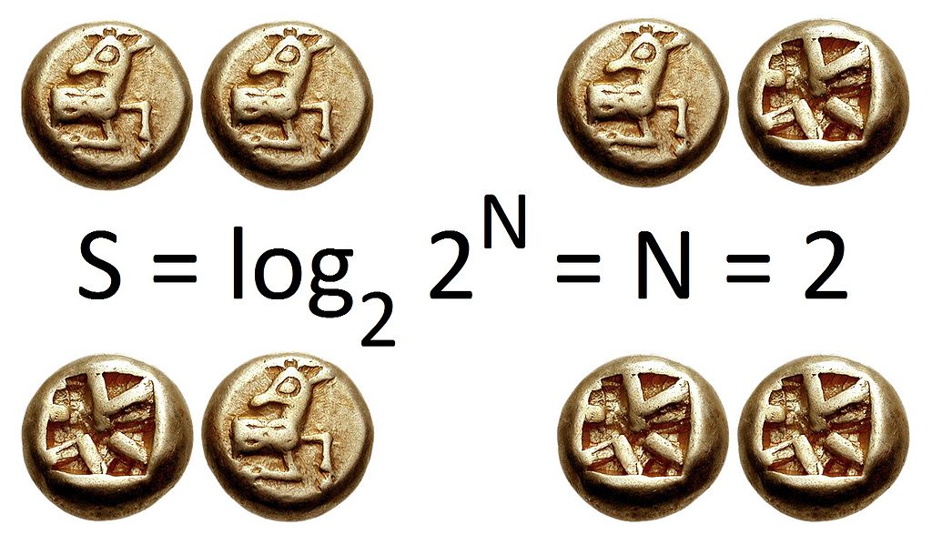
We’ve got two coins with two faces here. They can, obviously, be arranged in 2² = 4 ways. Now, back in 1948, the so-called father of information theory, Claude Shannon, thought it was nonsensical to just use that number (4) to represent the complexity of the situation. Indeed, if we’d take three coins, or four, or five, respectively, then we’d have 2³ = 8, 2⁴ = 16, and 2⁵ = 32 ways, respectively, of combining them. Now, you’ll agree that, as a measure of the complexity of the situation, the exponents 1, 2, 3, 4 etcetera describe the situation much better than 2, 4, 8, 16 etcetera.

Hence, Shannon defined the so-called information entropy as, in this case,  the base 2 logarithm of the number of possibilities. To be precise, the information entropy of the situation which we’re describing here (i.e. the ways a set of coins can be arranged) is equal to S = N = log₂(2^N) = 1, 2, 3, 4 etcetera for N = 1, 2, 3, 4 etcetera. In honor of Shannon, the unit is shannons. [I am not joking.] However, information theorists usually talk about bits, rather than shannons. [We’re not talking a computer bit here, although the two are obviously related, as computer bits are binary too.]

Now, one of the many nice things of logarithmic functions is that it’s easy to switch bases. Hence, instead of expressing information entropy in bits, we can also express it in trits (for base 3 logarithms), nats (for base e logarithms, so that’s the natural logarithmic function ln), or dits (for base 10 logarithms). So… Well… Feynman is right in noting that “the logarithm of the number of ways we can arrange the molecules is (the) entropy”, but that statement needs to be qualified: the concepts of information entropy and entropy tout court, as used in the context of thermodynamical analysis, are related but, as usual, they’re also different. 🙂 Bridging the two concepts involves probability distributions and other stuff. One extremely simple popular account illustrates the principle behind as follows:

Suppose that you put a marble in a large box, and shook the box around, and you didn’t look inside afterwards. Then the marble could be anywhere in the box. Because the box is large, there are many possible places inside the box that the marble could be, so the marble in the box has a high entropy. Now suppose you put the marble in a tiny box and shook up the box. Now, even though you shook the box, you pretty much know where the marble is, because the box is small. In this case we say that the marble in the box has low entropy.

Frankly, examples like this make only very limited sense. They may, perhaps, help us imagine, to some extent, how probability distributions of atoms or molecules might change as the atoms or molecules get more space to move around in. Having said that, I should add that examples like this are, at the same time, also so simplistic they may confuse us more than they enlighten us. In any case, while all of this discussion is highly relevant to statistical mechanics and thermodynamics, I am afraid I have to leave it at this one or two remarks. Otherwise this post risks becoming a course! 🙂

Now, there is one more thing we should talk about here. As you’ve read a lot of popular science books, you probably know that the temperature of the Universe is decreasing because it is expanding. However, from what you’ve learnt so far, it is hard to see why that should be the case. Indeed, it is easy to see why the temperature should drop/increase when there’s adiabatic expansion/compression: momentum and, hence, kinetic energy, is being transferred from/to the piston indeed, as it moves out or into the cylinder while the gas expands or is being compressed. But the expanding universe has nothing to push against, does it? So why should its temperature drop? It’s only the volume that changes here, right? And so its entropy (S) should increase, in line with the ΔS = S_b – S_a = S(V_b, T) – S(V_a, T) = ΔS = N·k·ln[V_b/V_a] formula, but not its temperature (T), which is nothing but the (average) kinetic energy of all of the particles it contains. Right? Maybe.

[By the way, in case you wonder why we believe the Universe is expanding, that’s because we see it expanding: an analysis of the redshifts and blueshifts of the light we get from other galaxies reveals the distance between galaxies is increasing. The expansion model is often referred to as the raisin bread model: one doesn’t need to be at the center of the Universe to see all others move away: each raisin in a rising loaf of raisin bread will see all other raisins moving away from it as the loaf expands.]

Why is the Universe cooling down?

This is a complicated question and, hence, the answer is also somewhat tricky. Let’s look at the entropy formula for an increasing volume of gas at constant temperature once more. Its entropy must change as follows:

ΔS = S_b – S_a = S(V_b, T) – S(V_a, T) = ΔS = N·k·ln[V_b/V_a]

Now, the analysis usually assumes we have to add some heat to the gas as it expands in order to keep the temperature (T) and, hence, its internal energy (U) constant. Indeed, you may or may not remember that the internal energy is nothing but the product of the number of gas particles and their average kinetic energy, so we can write:

U = N<mv²/2>

In my previous post, I also showed that, for an ideal gas (i.e. no internal motion inside of the gas molecules), the following equality holds: PV = (2/3)U. For a non-ideal gas, we’ve got a similar formula, but with a different coefficient: PV = (γ−1)U. However, all these formulas were based on the assumption that ‘something’ is containing the gas, and that ‘something’ involves the external environment exerting a force on the gas, as illustrated below.

As Feynman writes: “Suppose there is nothing, a vacuum, on the outside of the piston. What of it? If the piston were left alone, and nobody held onto it, each time it got banged it would pick up a little momentum and it would gradually get pushed out of the box. So in order to keep it from being pushed out of the box, we have to hold it with a force F.” We know that the pressure is the force per unit area: P = F/A. So can we analyze the Universe using these formulas?

Maybe. The problem is that we’re analyzing limiting situations here, and that we need to re-examine our concepts when applying them to the Universe. 🙂

The first question, obviously, is about the density of the Universe. You know it’s close to a vacuum out there. Close. Yes. But how close? If you google a bit, you’ll find lots of hard-to-read articles on the density of the Universe. If there’s one thing you need to pick up from them, is that, in order for the Universe to expand forever, it should have some critical density (denoted by ρ_c), which is like a watershed point between an expanding and a contracting Universe.

So what about it? According to Wikipedia, the critical density is estimated to be approximately five atoms (of monatomic hydrogen) per cubic metre, whereas the average density of (ordinary) matter in the Universe is believed to be 0.2 atoms per cubic metre. So that’s OK, isn’t it?

Well… Yes and no. We also have non-ordinary matter in the Universe, which is usually referred to as dark matter in the Universe. The existence of dark matter, and its properties, are inferred from its gravitational effects on visible matter and radiation. In addition, we’ve got dark energy as well. I don’t know much about it, but it seems the dark energy and the dark matter bring the actual density (ρ) of the Universe much closer to the critical density. In fact, cosmologists seem to agree thatρ ≈ ρ_c and, according to a very recent scientific research mission involving an ESA space observatory doing very precise measurements of the Universe’s cosmic background radiation, the Universe should consist of 4.82 ± 0.05% ordinary matter,25.8 ± 0.4% dark matter and 69 ± 1% dark energy. I’ll leave it to you to challenge that. 🙂

OK. Very low density. So that means very low pressure obviously. But what’s the temperature? I checked on the Physics Stack Exchange site, and the best answer is pretty nuanced: it depends on what you want to average. To be precise, the quoted answer is:

1. If one averages by volume, then one is basically talking about the ‘temperature’ of the photons that reach us as cosmic background radiation—which is the temperature of the Universe that those popular science books refer to. In that case, we get an average temperature of 2.72 degrees Kelvin. So that’s pretty damn cold!
2. If we average by observable mass, then our measurement is focused mainly on the temperature of all of the hydrogen gas (most matter in the Universe is hydrogen), which has a temperature of a few 10s of Kelvin. Only one tenth of that mass is in stars, but their temperatures are far higher: in the range of 10⁴to 10⁵ degrees. Averaging gives a range of 10³ to 10⁴ degrees Kelvin. So that’s pretty damn hot!
3. Finally, including dark matter and dark energy, which is supposed to have even higher temperature, we’d get an average by total mass in the range of 10⁷ Kelvin. That’s incredibly hot!

This is enlightening, especially the first point: we’re not measuring the average kinetic energy of matter particles here but some average energy of (heat) radiation per unit volume. This ‘cosmological’ definition of temperature is quite different from the ‘physical’ definition that we have been using and the observation that this ‘temperature’ must decrease is quite logical: if the energy of the Universe is a constant, but its volume becomes larger and larger as the Universe expands, then the energy per unit volume must obviously decrease.

So let’s go along with this definition of ‘temperature’ and look at an interesting study of how the Universe is supposed to have cooled down in the past. It basically measures the temperature of that cosmic background radiation, i.e. a remnant of the Big Bang, a few billion years ago, which was a few degrees warmer then than it is now. To be precise, it was measured as 5.08 ± 0.1 degrees Kelvin, and this decrease has nothing to do with our simple ideal gas laws but with the Big Bang theory, according to which the temperature of the cosmic background radiation should, indeed, drop smoothly as the universe expands.

Going through the same logic but the other way around, if the Universe had the same energy at the time of the Big Bang, it was all focused in a very small volume. Now, very small volumes are associated with very small entropy according to that S(V, T) = N·k·[ln(V) + ln(T)/(γ–1)] + a formula, but then temperature was not the same obviously: all that energy has to go somewhere, and a lot of it was obviously concentrated in the kinetic energy of its constituent particles (whatever they were) and, hence, a lot of it was in their temperature. 

So it all makes sense now. It was good to check out it out, as it reminds us that we should not try to analyze the Universe as a simple of body of gas that’s not contained in anything in order to then apply our equally simple ideal gas formulas. Our approach needs to be much more sophisticated. Cosmologists need to understand physics (and thoroughly so), but there’s a reason why it’s a separate discipline altogether. 🙂

Some content on this page was disabled on June 17, 2020 as a result of a DMCA takedown notice from Michael A. Gottlieb, Rudolf Pfeiffer, and The California Institute of Technology. You can learn more about the DMCA here:

https://en.support.wordpress.com/copyright-and-the-dmca/
Some content on this page was disabled on June 17, 2020 as a result of a DMCA takedown notice from Michael A. Gottlieb, Rudolf Pfeiffer, and The California Institute of Technology. You can learn more about the DMCA here:

https://en.support.wordpress.com/copyright-and-the-dmca/
Some content on this page was disabled on June 17, 2020 as a result of a DMCA takedown notice from Michael A. Gottlieb, Rudolf Pfeiffer, and The California Institute of Technology. You can learn more about the DMCA here:

https://en.support.wordpress.com/copyright-and-the-dmca/
Some content on this page was disabled on June 17, 2020 as a result of a DMCA takedown notice from Michael A. Gottlieb, Rudolf Pfeiffer, and The California Institute of Technology. You can learn more about the DMCA here:

https://en.support.wordpress.com/copyright-and-the-dmca/
Some content on this page was disabled on June 17, 2020 as a result of a DMCA takedown notice from Michael A. Gottlieb, Rudolf Pfeiffer, and The California Institute of Technology. You can learn more about the DMCA here:

https://en.support.wordpress.com/copyright-and-the-dmca/
Some content on this page was disabled on June 17, 2020 as a result of a DMCA takedown notice from Michael A. Gottlieb, Rudolf Pfeiffer, and The California Institute of Technology. You can learn more about the DMCA here:

https://en.support.wordpress.com/copyright-and-the-dmca/