The Ideal versus the Actual Gas Law

Pre-script (dated 26 June 2020): This post has become less relevant (even irrelevant, perhaps) because my views on all things quantum-mechanical have evolved significantly as a result of my progression towards a more complete realist (classical) interpretation of quantum physics. The text also got mutilated because of the removal of material by the dark force. I keep blog posts like these mainly because I want to keep track of where I came from. I might review them one day, but I currently don’t have the time or energy for it. 🙂

Original post:

In previous posts, we referred, repeatedly, to the so-called ideal gas law, for which we have various expressions. The expression we derived from analyzing the kinetics involved when individual gas particles (atoms or molecules) move and collide was P·V = N·k·T, in which the variables are P (pressure), V (volume), N (the number of particles in the given volume), T (temperature) and k (the Boltzmann constant). We also wrote it as P·V = (2/3)·U, in which U represents the total energy, i.e. the sum of the energies of all gas particles. We also said the P·V = (2/3)·U formula was only valid for monatomic gases, in which case U is the kinetic energy of the center-of-mass motion of the atoms.

In order to provide some more generality, the equation is often written as P·V = (γ–1)·U. Hence, for monatomic gases, we have γ = 5/3. For a diatomic gas, we’ll also have vibrational and rotational kinetic energy. As we pointed out in a previous post, each independent direction of motion, i.e. each degree of freedom in the system, will absorb an amount of energy equal to k·T/2. For monatomic gases, we have three independent directions of motion (x, y, z) and, hence, the total energy U = 3·k·T/2 = (2/3)·U.

Finally, when we’re considering adiabatic expansion/compression only – so when we do not add or remove any heat to/from to the gas – we can also write the ideal gas law as PV^γ = C, with C some constant. [It is important to note that this PV^γ = C relation can be derived from the more general P·V = (γ–1)·U expression, but that the two expressions are not equivalent. Please have a look at the P.S. to this post on this, which shows how we get that PV^γ = constant expression, and talks a bit about its meaning.]

So what’s the gas law for diatomic gas, like O₂, i.e. oxygen? The key to the analysis of diatomic gases is, basically, a model which represents the oxygen molecule as two atoms connected by a spring, but with a force law that’s not as simplistic as Hooke’s law: we’re not looking at some linear force, but a force that’s referred to as a van der Waals force. The image below gives a vague idea of what that might imply. Remember: when moving an object in a force field, we change its potential energy, and the work done, as we move with or against the force, is equal to the change in potential energy. The graph below shows the force is anything but linear.

The illustration above is a graph of potential energy for two molecules, but we can also apply it for the ‘spring’ model for two atoms within a single molecule. For the detail, I’ll refer you to Feynman’s Lecture on this. It’s not that the full story is too complicated: it’s just too lengthy to reproduce it in this post. Just note the key point of the whole story: one arrives at a theoretical value for γ that is equal to γ = 9/7 ≈ 1.286. Wonderful! Yes. Except for the fact that value does not correspond to what is measured in reality: the experimentally confirmed value for γ for oxygen (O₂) is about 1.40.

What about other gases? When measuring the value for other diatomic gases, like iodine (I₂) or bromine (Br₂), we get a value closer to the theoretical value (1.30 and 1.32 respectively) but, still, there’s a variation to be explained here. The value for hydrogen H₂ is about 1.4, so that’s like oxygen again. For other gases, we again get different values. Why? What’s the problem?

It cannot be explained using classical theory. In addition, doing the measurements for oxygen and hydrogen at various temperatures also reveals that γ is a function of temperature, as shown below. Now that’s another experimental fact that does not line up with our kinetic theory of gases!

Reality is right, always. Hence, our theory must be wrong. Our analysis of the independent direction of motions inside of a molecule doesn’t work—even for the simple case of a diatomic molecule. Great minds such as James Clerk Maxwell couldn’t solve the puzzle in the 19th century and, hence, had to admit classical theory was in trouble. Indeed, popular belief has it that the black-body radiation problem was the only thing classical theory couldn’t explain in the late 19th century but that’s not true: there were many more problems keeping physicists awake. But so we’ve got a problem here. As Feynman writes: “We might try some force law other than a spring but it turns out that anything else will only make γ higher. If we include more forms of energy, γ approaches unity more closely, contradicting the facts. All the classical theoretical things that one can think of will only make it worse. The fact is that there are electrons in each atom, and we know from their spectra that there are internal motions; each of the electrons should have at least kT/2 of kinetic energy, and something for the potential energy, so when these are added in, γ gets still smaller. It is ridiculous. It is wrong.”

So what’s the answer? The answer is to be found in quantum mechanics. Indeed, one can develop a model distinguishing various molecular states with various energy levels E₀, E₁, E₂,…, E_i,…, and then associate a probability distribution which gives us the probability of finding a molecule in a particular state. Some more assumptions, all quite similar to the assumptions used by Planck when he solved the black-body radiation problem, then give us what we want: to put it simply, it is like some of the motions ‘freeze out’ at lower temperatures. As a result, γ goes up as we go down in temperature.

Hence, quantum mechanics saves the day, again. However, that’s not what I want to write about here. What I want to do here is to give you an equation for the internal energy of a gas which is based on what we can actually measure, so that’s pressure, volume and temperature. I’ll refer to it as the Actual Gas Law, because it takes into account that γ is not some fixed value (so it’s not some natural constant, like Planck’s or Boltzmann’s constant), and it also takes into account that we’re not always gas—ideal or actual gas—but also liquids and solids.

Now, we have many inter-connected variables here, and so the analysis is quite complicated. In fact, it’s a great opportunity to learn more about partial derivatives and how we can use them. So the lesson is as much about math as it about physics. In fact, it’s probably more about math. 🙂 Let’s see what we can make out of it.

Energy, work, force, pressure and volume

First, I should remind you that work is something that is done by a force on some object in the direction of the displacement of that object. Hence, work is force times distance. Now, because the force may actually vary as our object is being displaced and while the work is being done, we represent work as a line integral:

W = ∫F·ds

We write F and s in bold-face and, hence, we’ve got a vector dot product here, which ensures we only consider the component of the force in the direction of the displacement: F·Δs = |F|·|Δs|·cosθ, with θ the angle between the force and the displacement.

As for the relationship between energy and work, you know that one: as we do work on an object, we change its energy, and that’s what we are looking at here: the (internal) energy of our substance. Indeed, when we have a volume of gas exerting pressure, it’s the same thing: some force is involved (pressure is the force per unit area, so we write: P = F/A) and, using the model of the box with the frictionless piston (illustrated below), we write:

dW = F(–dx) = – PAdx = – PdV

The dW = – PdV formula is the one we use when looking at infinitesimal changes. When going through the full thing, we should integrate, as the volume (and the pressure) changes over the trajectory, so we write:

W = ∫PdV

Now, it is very important to note that the formulas above (dW = – PdV and W = ∫PdV) are always valid. Always? Yes. We don’t care whether or not the compression (or expansion) is adiabatic or isothermal. [To put it differently, we don’t care whether or not heat is added to (or removed from) the gas as it expands (or decreases in volume).] We also don’t keep track of the temperature here. It doesn’t matter. Work is work.

Now, as you know, an integral is some area under a graph so I can rephrase our result as follows: the work that is being done by a gas, as it expands (or the work that we need to put in in order to compress it), is the area under the pressure-volume graph, always.

Of course, as we go through a so-called reversible cycle, getting work out of it, and then putting some work back in, we’ll have some overlapping areas cancelling each other. That’s how we derived the amount of useful (i.e. net) work that can be done by an ideal gas engine (illustrated below) as it goes through a Carnot cycle, taking in some amount of heat Q₁ from one reservoir (which is usually referred to as the boiler) and delivering some other amount of heat (Q₁) to another reservoir (usually referred to as the condenser). As I don’t want to repeat myself too much, I’ll refer you to one of my previous posts for more details. Hereunder, I just present the diagram once again. If you want to understand anything of what follows, you need to understand it—thoroughly.

It’s important to note that work is being done in each of the four steps of the cycle, and that the work done by the gas is positive when it expands, and negative when its volume is being reduced. So, let me repeat: the W = ∫PdV formula is valid for both adiabatic as well as isothermal expansion/compression. We just need to be careful about the sign and see in which direction it goes. Having said that, it’s obvious adiabatic and isothermal expansion/compression are two very different things and, hence, their impact on the (internal) energy of the gas is quite different:

1. Adiabatic compression/expansion assumes that no (external) heat energy (Q) is added or removed and, hence, all the work done goes into changing the internal energy (U). Hence, we can write: W = PΔV = –ΔU and, therefore, ΔU = –PΔV. Of course, adiabatic compression/expansion must involve a change in temperature, as the kinetic energy of the gas molecules is being transferred from/to the piston. Hence, the temperature (which is nothing but the average kinetic energy of the molecules) changes.
2. In contrast, isothermal compression/expansion (i.e. a volume change without any change in temperature) must involve an exchange of heat energy with the surroundings so to allow the temperature to remain constant. So ΔQ ≠ 0 in this case.

The grand but simple formula capturing all is, obviously:

ΔU = ΔQ – PΔV

It says what we’ve said already: the internal energy of a substance (a gas) changes because some work is being done as its volume changes and/or because some heat is added or removed.

Now we have to get serious about partial derivatives, which relate one variable (the so-called ‘dependent’ variable) to another (the ‘independent’ variable). Of course, in reality, all depends on all and, hence, the distinction is quite artificial. Physicists tend to treat temperature and volume as the ‘independent’ variables, while chemists seem to prefer to think in terms of pressure and temperature. In math, it doesn’t matter all that much: we simply take the reciprocal and there you go: dy/dx = 1/(dx/dy). We go from one to another. Well… OK… We’ve got a lot of variables here, so… Yes. You’re right. It’s not going to be that simple, obviously! 🙂

Differential analysis

If we have some function f in two variables, x and y, then we can write: Δf = f(x + Δx, y + Δy) –  f(x, y). We can then write the following clever thing:

What’s being said here is that we can approximate Δf using the partial derivatives ∂f/∂x and ∂f/∂y. Note that the formula above actually implies that we’re evaluating the (partial) ∂f/∂x derivative at point (x, y+Δy), rather than the point (x, y) itself. It’s a minor detail, but I think it’s good to signal it: this ‘clever thing’ is just pedagogical. [Feynman is the greatest teacher of all times! :-)] The mathematically correct approach is to simply give the formal definition of partial derivatives, and then just get on with it:

Now, let us apply that Δf formula to what we’re interested in, and that’s the change in the (internal) energy U. So we write:

Now, we can’t do anything with this, in practice, because we cannot directly measure the two partial derivatives. So, while this is an actual gas law (which is what we want), it’s not a practical one, because we can’t use it. 🙂 Let’s see what we can do about that. We need to find some formula for those partial derivatives. Let’s have a look at the (∂U/∂T)_V factor first. That factor is defined and referred to as the specific heat capacity at constant volume, and it’s usually denoted by C_V. Hence, we write:

C_V = specific heat capacity at constant volume = (∂U/∂T)_V

Heat capacity? But we’re talking internal energy here? It’s the same. Remember that ΔU = ΔQ – PΔV formula: if we keep the volume constant, then ΔV = 0 and, hence, ΔU = ΔQ. Hence, all of the change in internal energy (and I really mean all of the change) is the heat energy we’re adding or removing from the gas. Hence, we can also write C_V in its more usual definitional form:

C_V = (∂Q/∂T)_V

As for its interpretation, you should look at it as a ratio: C_V is the amount of heat one must put into (or remove from) a substance in order to change its temperature by one degree with the volume held constant. Note that the term ‘specific heat capacity’ is usually referred to as the ‘specific heat’, as that’s shorter and simpler. However, you can see it’s some kind of ‘capacity’ indeed. More specifically, it’s a capacity of a substance to absorb heat. Now that’s stuff we can actually measure and, hence, we’re done with the first term in that ΔU = ΔT·(∂U/∂T)_V + ΔV·(∂U/∂V)_T expression, which we can now write as:

ΔT·(∂U/∂T)_V = ΔT·(∂Q/∂T)_V = ΔT·C_V

OK. So we’re done with the first term. Just to make sure we’re on the right track here, let’s have a quick look at the units here: the unit in which we should measure C_V is, obviously, joule per degree (Kelvin), i.e. J/K. And then we multiply with ΔT, which is measured in degrees Kelvin, and we get some amount in Joule. Fine. We’re done, indeed. 🙂

Let’s look at the second term now, i.e. the ΔV·(∂U/∂V)_T term. Now, you may think that we could define C_T = (∂U/∂V)_T as the specific heat capacity at constant temperature because… Well… Hmm… It is the amount of heat one must put into (or remove from) a substance in order to change its volume by one unit with the temperature held constant, isn’t it? So we write C_T = (∂U/∂V)_T = (∂Q/∂V)_T and we’re done here too, aren’t we?

NO! HUGE MISTAKE!

It’s not that simple. Two very different things are happening here. Indeed, the change in (internal) energy ΔU, as the volume changes by ΔV while keeping the temperature constant (we’re looking at that (∂U/∂V)_T factor here, and I’ll remind you of that subscript T a couple of times), consists of two parts:

1. First, the volume is not being kept constant and, hence, the internal energy (U) changes because work is being done.
2. Second, the internal energy (U) also changes because heat is being put in, so the temperature can be kept constant indeed.

So we cannot simplify. We’re stuck with the full thing: ΔU = ΔQ – PΔV, in which – PΔV is the (infinitesimal amount of) work that’s being done on the substance, and ΔQ is the (infinitesimal amount of) heat that’s being put in. What can we do? How can we relate this to actual measurables?

Now, the logic is quite abstruse, so please be patient and bear with me. The key to the analysis is that diagram of the reversible Carnot cycle, with the shaded area representing the net work that’s being done, except that we’re now talking infinitesimally small changes in volume, temperature and pressure. So we redraw the diagram and get something like this:

Now, you can easily see the equivalence between the shaded area and the ΔPΔV rectangle below:

So the work done by the gas is the shaded area, whose surface is equal to ΔPΔV. […] But… Hey, wait a minute! You should object: we are not talking ideal engines here and, hence, we are not going through a full Carnot cycle, are we? We’re calculating the change in internal energy when the temperature changes with ΔT, the volume changes with ΔV, and the pressure changes with ΔP. Full stop. So we’re not going back to where we came from and, hence, we should not be analyzing this thing using the Carnot cycle, should we? Well… Yes and no. More yes than no. Remember we’re looking at the second term only here: ΔV·(∂U/∂V)_T. So we are changing the volume (and, hence, the internal energy) but the subscript in the (∂U/∂V)_T term makes it clear we’re doing so at constant temperature. In practice, that means we’re looking at a theoretical situation here that assumes a complete and fully reversible cycle indeed. Hence, the conceptual idea is, indeed, that we put some heat in, that the gas does some work as it expands, and that we then are actually putting some work back in to bring the gas back to its original temperature T. So, in short, yes, the reversible cycle idea applies.

[…] I know, it’s very confusing. I am actually struggling with the analysis myself, so don’t be too hard on yourself. Think about it, but don’t lose sleep over it. 🙂 I added a note on it in the P.S. to this post on it so you can check that out too. However, I need to get back to the analysis itself here. From our discussion of the Carnot cycle and ideal engines, we know that the work done is equal to the difference between the heat that’s being put in and the heat that’s being delivered: W = Q₁ – Q₂. Now, because we’re talking reversible processes here, we also know that Q₁/T₁ = Q₂/T₂. Hence, Q₂ = (T ₂/T₁)Q₁ and, therefore, the work done is also equal to W = Q₁ – (T ₂/T₁)Q₁ = Q₁(1 – T ₂/T₁) = Q₁[(T₁ – T₂)/T₁]= Q₁(ΔT/T₁). Let’s now drop the subscripts by equating Q₁ with ΔQ, so we have:

W = ΔQ(ΔT/T)

You should note that ΔQ is not the difference between Q₁ and Q₂. It is not. ΔQ is the heat we put in as it expands isothermally from volume V to volume V + ΔV. I am explicit about it because the Δ symbol usually denotes some difference between two values. In case you wonder how we can do away with Q₂, think about it. […] The answer is that we did not really get away with it: the information is captured in the ΔT factor, as T–ΔT is the final temperature reached by the gas as it expands adiabatically on the second leg of the cycle, and the change in temperature obviously depends on Q₂! Again, it’s all quite confusing because we’re looking at infinitesimal changes only, but the analysis is valid. [Again, go through the P.S. of this post if you want more remarks on this, although I am not sure they’re going to help you much. The logic is really very deep.]

[…] OK… I know you’re getting tired, but we’re almost done. Hang in there. So what do we have now? The work done by the gas as it goes through this infinitesimally small cycle is the shaded area in the diagram above, and it is equal to:

W = ΔPΔV = ΔQ(ΔT/T)

From this, it follows that ΔQ = T·ΔV·ΔP/ΔT. Now, you should look at the diagram once again to check what ΔP actually stands for: it’s the change in pressure when the temperature changes at constant volume. Hence, using our partial derivative notation, we write:

ΔP/ΔT = (∂P/∂T)_V

We can now write ΔQ = T·ΔV·(∂P/∂T)_V and, therefore, we can re-write ΔU = ΔQ – PΔV as:

ΔU = T·ΔV·(∂P/∂T)_V – PΔV

Now, dividing both sides by ΔV, and writing all using the partial derivative notation, we get:

ΔU/ΔV = (∂U/∂V)_T = T·(∂P/∂T)_V – P

So now we know how to calculate the (∂U/∂V)_T factor, from measurable stuff, in that ΔU = ΔT·(∂U/∂T)_V + ΔV·(∂U/∂V)_T expression, and so we’re done. Let’s write it all out:

ΔU = ΔT·(∂U/∂T)_V + ΔV·(∂U/∂V)_T = ΔT·C_V + ΔV·[T·(∂P/∂T)_V – P]

Phew! That was tough, wasn’t it? It was. Very tough. As far as I am concerned, this is probably the toughest of all I’ve written so far.

Dependent and independent variables 

Let’s pause to take stock of what we’ve done here. The expressions above should make it clear we’re actually treating temperature and volume as the independent variables, and pressure and energy as the dependent variables, or as functions of (other) variables, I should say. Let’s jot down the key equations once more:

1. ΔU = ΔQ – PΔV
2. ΔU = ΔT·(∂U/∂T)_V + ΔV·(∂U/∂V)_T 
3. (∂U/∂T)_V = (∂Q/∂T)_V = C_V
4. (∂U/∂V)_T = T·(∂P/∂T)_V – P

It looks like Chinese, doesn’t it? 🙂 What can we do with this? Plenty. Especially the first equation is really handy for analyzing and solving various practical problems. The second equation is much more difficult and, hence, less practical. But let’s try to apply this equation for actual gases to an ideal gas—just to see if we’re getting our ideal gas law once again. 🙂 We know that, for an ideal gas, the internal energy depends on temperature, not on V. Indeed, if we change the volume but we keep the temperature constant, the internal energy should be the same, as it only depends on the motion of the molecules and their number. Hence, (∂U/∂V)_T must equal zero and, hence, T·(∂P/∂T)_V – P = 0. Replacing the partial derivative with an ordinary one (not forgetting that the volume is kept constant), we get:

T·(dP/dT) – P = 0 (constant volume)

⇔ (1/P)·(dP/dT) = 1/T (constant volume)

Integrating both sides yields: lnP = lnT + constant. This, in turn, implies that P = T × constant. [Just re-write the first constant as the (natural) logarithm of some other constant, i.e. the second constant, obviously).] Now that’s consistent with our ideal gas P = NkT/V, because N, k and V are all constant. So, yes, the ideal gas law is a special case of our more general thermodynamical expression. Fortunately! 🙂

That’s not very exciting, you’ll say—and you’re right. You may be interested – although I doubt it 🙂 – in the chemists’ world view: they usually have performance data (read: values for derivatives) measured under constant pressure. The equations above then transform into:

1. ΔH = Δ(U + P·V) = ΔQ + VΔP
2. ΔH = ΔT·(∂H/∂T)_P + ΔP·(∂H/∂P)_T 
3. (∂H/∂P)_T = –T·(∂V/∂T)_P + V

H? Yes. H is another so-called state variable, so it’s like entropy or internal energy but different. As they say in Asia: “Same-same but different.” 🙂 It’s defined as H = U + PV and its name is enthalpy. Why do we need it? Because some clever man noted that, if you take the total differential of P·V, i.e. Δ(P·V) = P·ΔV + V·ΔP, and our ΔU = ΔQ – P·ΔV expression, and you add both sides of both expressions, you get Δ(U + P·V) = ΔQ + VΔP. So we’ve substituted –P for V – so as to please the chemists – and all our equations hold provided we substitute U for H and, importantly, –P for V. [Note the sign switch is to be applied to derivatives as well: if we substitute P for –V, then ∂P/∂T becomes ∂(–V)/∂T = –(∂V/∂T)!

So that’s the chemists’ model of the world, and they’ll usually measure the specific heat capacity at constant pressure, rather than at constant volume. Indeed, one can show the following:

(∂H/∂T)_P = (∂Q/∂T)_P = C_P = the specific heat capacity at constant pressure

In short, while we referred to γ as the specific heat ratio in our previous posts, assuming we’re talking ideal gases only, we can now appreciate the fact there is actually no such thing as the specific heat: there are various variables and, hence, various definitions. Indeed, it’s not only pressure or volume: the specific heat capacity of some substance will usually also be expressed as a function of its mass (i.e. per kg), the number of particles involved (i.e. per mole), or its volume (i.e. per m³). In that case, we talk about the molar or volumetric heat capacity respectively. The name for the same thing expressed in joule per degree Kelvin and per kg (J/kg·K) is the same: specific heat capacity. So we’ve got three different concepts here, and two ways of measuring them: at constant pressure or at constant volume. No wonder one gets quite confused when googling tables listing the actual values! 🙂

Now, there’s one question left: why is γ being referred to as the specific heat ratio? The answer is simple: it actually is the ratio of the specific heat capacities C_P and C_V. Hence, γ is equal to:

γ = C_P/C_V

I could show you how that works. However, I would just be copying the Wikipedia article on it, so I won’t do that: you’re sufficiently knowledgeable now to check it out yourself, and verify it’s actually true. Good luck with it ! In the process, please also do check why C_P is always larger than C_V so you can explain why γ is always larger than one. 🙂

Post scriptum: As usual, Feynman’s Lectures, were the inspiration here—once more. Now, Feynman has a habit of ‘integrating’ expressions and, frankly, I never found a satisfactory answer to a pretty elementary question: integration in regard to what variable? His exposé on both the ideal as well as the actual gas law has enlightened me. The answer is simple: it doesn’t matter. 🙂 Let me show that by analyzing the following argument of Feynman:

So… What is that ‘integration’ that ‘yields’ that γlnV + lnP = lnC expression? Are we solving some differential equation here? Well… Yes. But let’s be practical and take the derivative of the expression in regard to V, P and T respectively. Let’s first see where we come from. The fundamental equation is PV = (γ–1)U. That means we’ve got two ‘independent’ variables, and one that ‘depends’ on the others: if we fix P and V, we have U, or if we fix U, then P and V are in an inversely proportional relationship. That’s easy enough. We’ve got three ‘variables’ here: U, P and V—or, in differential form, dU, dP and dV. However, Feynman eliminates one by noting that dU = –PdV. He rightly notes we can only do that because we’re talking adiabatic expansion/compression here: all the work done while expanding/compressing the gas goes into changing the internal energy: no heat is added or removed. Hence, there is no dQ term here.

So we are left with two ‘variables’ only now: P and V, or dP and dV when talking differentials. So we can choose: P depends on V, or V depends on P. If we think of V as the independent variable, we can write:

d[γ·lnV + lnP]/dV = γ·(1/V)·(dV/dV) + (1/P)·(dP/dV), while d[lnC]/dV = 0

So we have γ·(1/V)·(dV/dV) + (1/P)·(dP/dV) = 0, and we can then multiply sides by dV to get:

(γ·dV/V) + (dP/P) = 0,

which is the core equation in this argument, so that’s the one we started off with. Picking P as the ‘independent’ variable and, hence, integrating with respect to P yields the same:

d[γ·lnV + lnP]/dP = γ·(1/V)·(dV/dP) + (1/P)·(dP/dP), while d[lnC]/dP = 0

Multiplying both sides by dP yields the same thing: (γ·dV/V) + (dP/P) = 0. So it doesn’t matter, indeed. But let’s be smart and assume both P and V, or dP and dV, depend on some implicit variable—a parameter really. The obvious candidate is temperature (T). So we’ll now integrate and differentiate in regard to T. We get:

d[γ·lnV + lnP]/dT = γ·(1/V)·(dV/dT) + (1/P)·(dP/dT), while d[lnC]/dT = 0

We can, once again, multiply both sides with dT and – surprise, surprise! – we get the same result: 

(γ·dV/V) + (dP/P) = 0

The point is that the γlnV + lnP = lnC expression is damn valid, and C or lnC or whatever is ‘the constant of integration’ indeed, in regard to whatever variable: it doesn’t matter. So then we can, indeed, take the exponential of both sides (which is much more straightforward than ‘integrating both sides’), so we get:

e^{γlnV + lnP} = e^lnC = C

It then doesn’t take too much intelligence to see that e^{γlnV + lnP} = e^(lnV)γ+lnP = e^(lnV)γ·e^lnP = V^γ·P = P·V^γ. So we’ve got the grand result that what we wanted: PV^γ = C, with C some constant determined by the situation we’re in (think of the size of the box, or the density of the gas).

So, yes, we’ve got a ‘law’ here. We should just remind ourselves, always, that it’s only valid when we’re talking adiabatic compression or expansion: so we we do not add or remove heat energy or, as Feynman puts it, much more succinctly, “no heat is being lost“. And, of course, we’re also talking ideal gases only—which excludes a number of real substances. 🙂 In addition, we’re talking adiabatic processes only: we’re not adding nor removing heat.

It’s a weird formula: the pressure times the volume to the 5/3 power is a constant for monatomic gas. But it works: as long as individual atoms are not bound to each other, the law holds. As mentioned above, when various molecular states, with associated energy levels are at play, it becomes an entirely different ballgame. 🙂

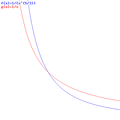
I should add one final note as to the functional form of PV^γ = C. We can re-write it as P = C/V^γ. Because The shape of that graph is similar to the P = NkT/V relationship we started off with. Putting the two equations side by side, makes it clear our constant and temperature are obviously related one to another, but they are not directly proportional to each other. In fact, as the graphs below clearly show, the P = NkT/V gives us these isothermal lines on the pressure-volume graph (i.e. they show P and V are related at constant temperature), while the P = C/V^γ equation gives us the adiabatic lines. Just google an online function graph tool, and you can now draw your own diagrams of the Carnot cycle! Just change the denominator (i.e. the constants C and T in both equations). 🙂

Now, I promised I would say something more about that infinitesimal Carnot cycle: why is it there? Why don’t we limit the analysis to just the first two steps? In fact, the shortest and best explanation I can give is something like this: think of the whole cycle as the first step in a reversible process really. We put some heat in (ΔQ) and the gas does some work, but so that heat has to go through the whole body of gas, and the energy has to go somewhere too. In short, the heat and the work is not being absorbed by the surroundings but it all stays in the ‘system’ that we’re analyzing, so to speak, and that’s why we’re going through the full cycle, not the first two steps only. Now, this ‘answer’ may or may not satisfy you, but I can’t do better. You may want to check Feynman’s explanation itself, but he’s very short on this and, hence, I think it won’t help you much either. 😦

Some content on this page was disabled on June 16, 2020 as a result of a DMCA takedown notice from The California Institute of Technology. You can learn more about the DMCA here:

https://en.support.wordpress.com/copyright-and-the-dmca/
Some content on this page was disabled on June 16, 2020 as a result of a DMCA takedown notice from The California Institute of Technology. You can learn more about the DMCA here:

https://en.support.wordpress.com/copyright-and-the-dmca/
Some content on this page was disabled on June 17, 2020 as a result of a DMCA takedown notice from Michael A. Gottlieb, Rudolf Pfeiffer, and The California Institute of Technology. You can learn more about the DMCA here:

https://en.support.wordpress.com/copyright-and-the-dmca/
Some content on this page was disabled on June 17, 2020 as a result of a DMCA takedown notice from Michael A. Gottlieb, Rudolf Pfeiffer, and The California Institute of Technology. You can learn more about the DMCA here:

https://en.support.wordpress.com/copyright-and-the-dmca/
Some content on this page was disabled on June 17, 2020 as a result of a DMCA takedown notice from Michael A. Gottlieb, Rudolf Pfeiffer, and The California Institute of Technology. You can learn more about the DMCA here:

https://en.support.wordpress.com/copyright-and-the-dmca/