Feynman’s Seminar on Superconductivity (1)

Pre-script (dated 26 June 2020): This post got mutilated by the removal of some material by the dark force. You should be able to follow the main story line, however. If anything, the lack of illustrations might actually help you to think things through for yourself. In any case, we now have different views on these concepts as part of our realist interpretation of quantum mechanics, so we recommend you read our recent papers instead of these old blog posts.

Original post:

The ultimate challenge for students of Feynman’s iconic Lectures series is, of course, to understand his final one: A Seminar on Superconductivity. As he notes in his introduction to this formidably dense piece, the text does not present the detail of each and every step in the development and, therefore, we’re not supposed to immediately understand everything. As Feynman puts it: we should just believe (more or less) that things would come out if we would be able to go through each and every step. Well… Let’s see. Feynman throws a lot of stuff in here—including, I suspect, some stuff that may not be directly relevant, but that he sort of couldn’t insert into all of his other Lectures. So where do we start?

It took me one long maddening day to figure out the first formula:It says that the amplitude for a particle to go from a to b in a vector potential (think of a classical magnetic field) is the amplitude for the same particle to go from a to b when there is no field (A = 0) multiplied by the exponential of the line integral of the vector potential times the electric charge divided by Planck’s constant. I stared at this for quite a while, but then I recognized the formula for the magnetic effect on an amplitude, which I described in my previous post, which tells us that a magnetic field will shift the phase of the amplitude of a particle with an amount equal to:

Hence, if we write 〈b|a〉 for A = 0 as 〈b|a〉_{A = 0} = C·e^iθ, then 〈b|a〉 in A will, naturally, be equal to 〈b|a〉 _{in A} = C·e^i(θ+φ) = C·e^iθ·e^iφ = 〈b|a〉_{A = 0} ·e^iφ, and so that explains it. 🙂 Alright… Next. Or… Well… Let us briefly re-examine the concept of the vector potential, because we’ll need it a lot. We introduced it in our post on magnetostatics. Let’s briefly re-cap the development there. In Maxwell’s set of equations, two out of the four equations give us the magnetic field: ∇•B = 0 and c²∇×B = j/ε₀. We noted the following in this regard:

1. The ∇•B = 0 equation is true, always, unlike the ∇×E = 0 expression, which is true for electrostatics only (no moving charges). So the ∇•B = 0 equation says the divergence of B is zero, always.
2. The divergence of the curl of a vector field is always zero. Hence, if A is some vector field, then div(curl A) = ∇•(∇×A) = 0, always.
3. We can now apply another theorem: if the divergence of a vector field, say D, is zero—so if ∇•D = 0—then D will be the the curl of some other vector field C, so we can write: D = ∇×C.  Applying this to ∇•B = 0, we can write: 

If ∇•B = 0, then there is an A such that B = ∇×A

So, in essence, we’re just re-defining the magnetic field (B) in terms of some other vector field. To be precise, we write it as the curl of some other vector field, which we refer to as the (magnetic) vector potential. The components of the magnetic field vector can then be re-written as:

We need to note an important point here: the equations above suggest that the components of B depend on position only. In other words, we assume static magnetic fields, so they do not change with time. That, in turn, assumes steady currents. We will want to extend the analysis to also include magnetodynamics. It complicates the analysis but… Well… Quantum mechanics is complicated. Let us remind ourselves here of Feynman’s re-formulation of Maxwell’s equations as a set of two equations (expressed in terms of the magnetic (vector) and the electric potential) only:

These equations are wave equations, as you can see by writing out the second equation:

The Schrödinger equation in an electromagnetic field

Feynman then jots down Schrödinger’s equation for the same particle (with charge q) moving in an electromagnetic field that is characterized not only by the (scalar) potential Φ but also by a vector potential A:

Now where does that come from? We know the standard formula in an electric field, right? It’s the formula we used to find the energy states of electrons in a hydrogen atom:

i·ħ·∂ψ/∂t = −(1/2)·(ħ²/m)∇²ψ + V·ψ

Of course, it is easy to see that we replaced V by q·Φ, which makes sense: the potential of a charge in an electric field is the product of the charge (q) and the (electric) potential (Φ), because Φ is, obviously, the potential energy of the unit charge. It’s also easy to see we can re-write −ħ²·∇²ψ as [(ħ/i)·∇]·[(ħ/i)·∇]ψ because (1/i)·(1/i) = 1/i² = 1/(−1) = −1. 🙂 Alright. So it’s just that −q·A term in the (ħ/i)∇ − q·A expression that we need to explain now.

Unfortunately, that explanation is not so easy. Feynman basically re-derives Schrödinger’s equation using his trade-mark historical argument – which did not include any magnetic field – with a vector potential. The re-derivation is rather annoying, and I didn’t have the courage to go through it myself, so you should – just like me – just believe Feynman when he says that, when there’s a vector potential – i.e. when there’s a magnetic field – then that (ħ/i)·∇ operator – which is the momentum operator– ought to be replaced by a new momentum operator:

So… Well… There we are… 🙂 So far, so good? Well… Maybe.

While, as mentioned, you won’t be interested in the mathematical argument, it is probably worthwhile to reproduce Feynman’s more intuitive explanation of why the operator above is what it is. In other words, let us try to understand that −qA term. Look at the following situation: we’ve got a solenoid here, and some current I is going through it so there’s a magnetic field B. Think of the dynamics while we turn on this flux. Maxwell’s second equation (∇×E = −∂B/∂t) tells us the line integral of E around a loop will be equal to the time rate of change of the magnetic flux through that loop. The ∇×E = −∂B/∂t equation is a differential equation, of course, so it doesn’t have the integral, but you get the idea—I hope.

Now, using the B = ∇×A equation we can re-write the ∇×E = −∂B/∂t as ∇×E = −∂(∇×A)/∂t. This allows us to write the following:

 ∇×E = −∂(∇×A)/∂t = −∇×(∂A/∂t) ⇔ E = −∂A/∂t

This is a remarkable expression. Note its derivation is based on the commutativity of the curl and time derivative operators, which is a property that can easily be explained: if we have a function in two variables—say x and t—then the order of the derivation doesn’t matter: we can first take the derivative with respect to x and then to t or, alternatively, we can first take the time derivative and then do the ∂/∂x operation. So… Well… The curl is, effectively, a derivative with regard to the spatial variables. OK. So what? What’s the point?

Well… If we’d have some charge q, as shown in the illustration above, that would happen to be there as the flux is being switched on, it will experience a force which is equal to F = qE. We can now integrate this over the time interval (t) during which the flux is being built up to get the following:

∫₀^t F = ∫₀^t m·a = ∫₀^t m·dv/dt = m·v_t= ∫₀^t q·E = −∫₀^t q·∂A/∂t = −q·A_t

Assuming v₀ and A₀ are zero, we may drop the time subscript and simply write:

m·v = −q·A

The point is: during the build-up of the magnetic flux, our charge will pick up some (classical) momentum that is equal to p = m·v = −q·A. So… Well… That sort of explains the additional term in our new momentum operator.

Note: For some reason I don’t quite understand, Feynman introduces the weird concept of ‘dynamical momentum’, which he defines as the quantity m·v + q·A, so that quantity must be zero in the analysis above. I quickly googled to see why but didn’t invest too much time in the research here. It’s just… Well… A bit puzzling. I don’t really see the relevance of his point here: I am quite happy to go along with the new operator, as it’s rather obvious that introducing changing magnetic fields must, obviously, also have some impact on our wave equations—in classical as well as in quantum mechanics.

Local conservation of probability

The title of this section in Feynman’s Lecture (yes, still the same Lecture – we’re not switching topics here) is the equation of continuity for probabilities. I find it brilliant, because it confirms my interpretation of the wave function as describing some kind of energy flow. Let me quote Feynman on his endeavor here:

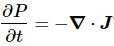
“An important part of the Schrödinger equation for a single particle is the idea that the probability to find the particle at a position is given by the absolute square of the wave function. It is also characteristic of the quantum mechanics that probability is conserved in a local sense. When the probability of finding the electron somewhere decreases, while the probability of the electron being elsewhere increases (keeping the total probability unchanged), something must be going on in between. In other words, the electron has a continuity in the sense that if the probability decreases at one place and builds up at another place, there must be some kind of flow between. If you put a wall, for example, in the way, it will have an influence and the probabilities will not be the same. So the conservation of probability alone is not the complete statement of the conservation law, just as the conservation of energy alone is not as deep and important as the local conservation of energy. If energy is disappearing, there must be a flow of energy to correspond. In the same way, we would like to find a “current” of probability such that if there is any change in the probability density (the probability of being found in a unit volume), it can be considered as coming from an inflow or an outflow due to some current.”

This is it, really ! The wave function does represent some kind of energy flow – between a so-called ‘real’ and a so-called ‘imaginary’ space, which are to be defined in terms of directional versus rotational energy, as I try to point out – admittedly: more by appealing to intuition than to mathematical rigor – in that post of mine on the meaning of the wavefunction.

So what is the flow – or probability current as Feynman refers to it? Well… Here’s the formula:

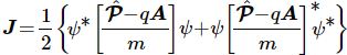
Huh? Yes. Don’t worry too much about it right now. The essential point is to understand what this current – denoted by J – actually stands for:

So what’s next? Well… Nothing. I’ll actually refer you to Feynman now, because I can’t improve on how he explains how pairs of electrons start behaving when temperatures are low enough to render Boltzmann’s Law irrelevant: the kinetic energy that’s associated with temperature can no longer break up electron pairs if temperature comes close to the zero point.

Huh? What? Electron pairs? Electrons are not supposed to form pairs, are they? They carry the same charge and are, therefore, supposed to repel each other. Well… Yes and no. In my post on the electron orbitals in a hydrogen atom – which just presented Feynman’s presentation on the subject-matter in a, hopefully, somewhat more readable format – we calculated electron orbitals neglecting spin. In Feynman’s words:

“We make another approximation by forgetting that the electron has spin. […] The non-relativistic Schrödinger equation disregards magnetic effects. [However] Small magnetic effects [do] occur because, from the electron’s point-of-view, the proton is a circulating charge which produces a magnetic field. In this field the electron will have a different energy with its spin up than with it down. [Hence] The energy of the atom will be shifted a little bit from what we will calculate. We will ignore this small energy shift. Also we will imagine that the electron is just like a gyroscope moving around in space always keeping the same direction of spin. Since we will be considering a free atom in space the total angular momentum will be conserved. In our approximation we will assume that the angular momentum of the electron spin stays constant, so all the rest of the angular momentum of the atom—what is usually called “orbital” angular momentum—will also be conserved. To an excellent approximation the electron moves in the hydrogen atom like a particle without spin—the angular momentum of the motion is a constant.”

To an excellent approximation… But… Well… Electrons in a metal do form pairs, because they can give up energy in that way and, hence, they are more stable that way. Feynman does not go into the details here – I guess because that’s way beyond the undergrad level – but refers to the Bardeen-Coopers-Schrieffer (BCS) theory instead – the authors of which got a Nobel Prize in Physics in 1972 (that’s a decade or so after Feynman wrote this particular Lecture), so I must assume the theory is well accepted now. 🙂

Of course, you’ll shout now: Hey! Hydrogen is not a metal! Well… Think again: the latest breakthrough in physics is making hydrogen behave like a metal. 🙂 And I am really talking the latest breakthrough: Science just published the findings of this experiment last month! 🙂 🙂 In any case, we’re not talking hydrogen here but superconducting materials, to which – as far as we know – the BCS theory does apply.

So… Well… I am done. I just wanted to show you why it’s important to work your way through Feynman’s last Lecture because… Well… Quantum mechanics does explain everything – although the nitty-gritty of it (the Meissner effect, the London equation, flux quantization, etc.) are rather hard bullets to bite. 😦

Don’t give up ! I am struggling with the nitty-gritty too ! 🙂

Some content on this page was disabled on June 16, 2020 as a result of a DMCA takedown notice from The California Institute of Technology. You can learn more about the DMCA here:

https://en.support.wordpress.com/copyright-and-the-dmca/
Some content on this page was disabled on June 16, 2020 as a result of a DMCA takedown notice from The California Institute of Technology. You can learn more about the DMCA here:

https://en.support.wordpress.com/copyright-and-the-dmca/
Some content on this page was disabled on June 16, 2020 as a result of a DMCA takedown notice from The California Institute of Technology. You can learn more about the DMCA here:

https://en.support.wordpress.com/copyright-and-the-dmca/
Some content on this page was disabled on June 16, 2020 as a result of a DMCA takedown notice from The California Institute of Technology. You can learn more about the DMCA here:

https://en.support.wordpress.com/copyright-and-the-dmca/
Some content on this page was disabled on June 16, 2020 as a result of a DMCA takedown notice from The California Institute of Technology. You can learn more about the DMCA here:

https://en.support.wordpress.com/copyright-and-the-dmca/
Some content on this page was disabled on June 16, 2020 as a result of a DMCA takedown notice from The California Institute of Technology. You can learn more about the DMCA here:

https://en.support.wordpress.com/copyright-and-the-dmca/