
Pre-script (dated 26 June 2020): This post got mutilated by the removal of some material by the dark force. You should be able to follow the main story line, however. If anything, the lack of illustrations might actually help you to think things through for yourself.
Original post:
Not all is exciting when studying physics. In fact, electromagnetism is, most of the time, a extremely boring subject-matter. But so we need to get through it, because we need the math and the formulas. So… Here we go… ![]()
When going from electrostatics to electrodynamics, one first needs to have a look at magnetostatics, to get familiar with (steady) electric currents. So let’s have a look at what they are. Of course, you already know what steady currents are. In that case, you should, perhaps, stop reading. But I’d recommend you go through it anyway. It’s always good to be explicit, so let’s be explicit.
Let me first make a very pedantic note. There are a couple of sections in Feynman’s Lectures in which he assumes that a steady current in a wire is uniformly distributed throughout the cross-section of the current-carrying wire: that assumption amounts to saying that the current density j is uniform. He uses that assumption, for example, when calculating the force per unit length of a current-carrying wire in a magnetic field (see Vol. II, section 13-3). He also uses it when calculating the magnetic field it creates itself (see Vol. II, section 14-3). This raises two questions:
- Is the assumption true?
- Does it matter?
My impression is that it’s a simplification that doesn’t matter. So the answer to both question would be negative. But let’s examine them. First note that, in previous posts, we repeatedly said that, if we place a charge Q on any conductor, all charges will spread out in some way on the surface, so we have an equipotential on the surface and no electric field inside of the conductor. The physics behind are easy to understand: if there were an electric field inside of the conductor, and the surface were not an equipotential, the charges would keep moving until it became zero.
Does it matter? Maybe. Maybe not. I discussed the electric field from a conductor in a previous post, so let me just recall some formulas here, first and foremost Gauss’ Law, which says that the electric flux from any closed surface S is equal to Qinside/ε0. Now, Qinside is, obviously, the sum of the charges inside the volume enclosed by the surface, and the most remarkable thing about Gauss’ Law is that the charge distribution inside of the volume doesn’t matter. So if we’re talking a uniformly charged sphere or a thin spherical shell of charge, it’s the same. The illustration below shows the field for a uniformly charged sphere: E is proportional to r (to be precise: E = (ρ·r)/(3ε0) for r ≤ R) inside the sphere, and outside E is proportional to 1/r2 (to be precise: E = Qinside/(4πε0r2) for r ≥ R).

However, Gauss’ Law is a law that gives us the electric flux only, so we’re talking E only. We also have the magnetic field, i.e. the field vector B. So what’s the equivalent of Gauss’ Law for B? That’s Ampère’s Law, obviously, so let’s have a look at how Feynman derives that law.
Ampère’s Law
Feynman starts by defining the current through some surface S as the following integral:
The illustration below explains the logic behind. The vector j is like the heat flow vector h which we used when explaining the basics of vector calculus: it is some amount passing expressed per unit time and per unit area. As for the use of n, that’s the same normal unit vector we used for h as well: we then wrote that h·n = |h|·|n|·cosθ = h·cosθ was the component of the heat flow that’s perpendicular or normal (as mathematicians prefer to say) to the surface. So here we’ve got the same: j·n·dS is the amount of charge flowing across an infinitesimally small area dS in a unit time. So to get the electric current I, which is the total charge passing per unit time through a surface S, we need to integrate the normal component of the flow through all the surface elements, which is what the integral above is doing.
Note that I is not a vector but a scalar. We could, however, include the idea of the direction of flow by making I a vector, so then we write it in boldface: I. It is measured in coulomb per second, aka as ampere: 1 A = 1 C/s. Also note we don’t have any wires here: just surfaces and volumes. 🙂 Onwards!
The equations of magnetostatics are Maxwell’s third and fourth equation and, as we used Maxwell’s first and second equation to derive Gauss’ Law, we’ll use these two to derive Ampère’s Law: (1) ∇•B = 0 and (2) c2∇×B = j/ε0.
You know these equations: the first one basically says there’s no flux of B: there’s no such thing as magnetic charges, in other words. The second one says that a current produces some circulation of B. You also know these equations are valid only for static fields: all electric charge densities are constant, and all currents are steady, so the electric and magnetic fields are not changing with time: ∂E/∂t = 0 = ∂B/∂t. Forget about c2 for a moment (it’s just a constant) and note that ∇×B is referred to as the curl of B.
Now, as I pointed out in one of my posts on vector analysis, the divergence of the curl of a vector is always equal to zero, so ∇•(∇×B) = 0. However, because ∇×B = j/ε0c2, that means ∇•(j/ε0c2) must also be equal to zero (we’re just taking the divergence of both sides of the equation here), and so we find that ∇•j must be equal to zero. What does that mean?Well… From the same post, you may or may not remember that the divergence of some vector field C (so that’s ∇•C) is the (net) flux out of an (infinitesimal) volume around the point we’re considering, so ∇•j = 0 implies that as much charge must be coming in as it going out, always and everywhere. So that means that, because of the charge conservation law (no charges are created or lost), we can only look at charges flowing in paths that close back on themselves, so we can only consider closed circuits. It’s a minor point – so don’t worry too much about it – but it does imply that we’re not looking at condensers, for example. Just remember: magnetostatics is about circulation, we have no flux, not of B, and not of j: our field, and our charges, circulate. 🙂
OK. Let’s get back to the lesson. We need to find Ampère’s Law, so we’d better get on with it. 🙂 To find Gauss’ Law, we used Gauss’ Theorem. To find Ampère’s Law, we’ll use… Stokes’ Theorem. [Sorry!] I need to refer you, once again, to that post on vector analysis for it. Here I can only remind you of the Theorem itself. It says that the line integral of the tangential component of a vector (field) around a closed loop is equal to the surface integral of the normal component of the curl of that vector over any surface which is bounded by the loop. […] I know that’s quite a mouthful, so let me jot down the equation:
Applying it to the magnetic field vector B, we get:
This is the illustration which goes with it.
Now, using our ∇×B = j/ε0c2 equation, we get:
Finally, we just plug in our I = ∫ j·n dS integral and we’re done. This is Ampère’s Law:
It basically says that the circulation of B around any closed curve is equal to the current I through the loop, divided by ε0c2. So what can we do with it? Well… We used Gauss’ Law to find the electric field in various circumstances, so let’s now use Ampère’s Law to find the magnetic field in various circumstances. 🙂
Before doing so, however, let me note that Ampère’s Law does not depend on any particular assumption in regard to the distribution of the charge densities j. So, frankly speaking, don’t worry too much about that assumption about a steady current in a wire: a current is a current in Ampère’s Law. 🙂
Wires
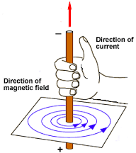
You know the magnetic field around a wire, as you’ll surely remember that right-hand rule for it from your high-school physics classes. Note, however, that it assumes you apply the usual convention: charge flows from positive to negative, because our unit of electric charge is obviously +1, not –1. So the electron flow actually goes the other way. 🙂
But so we’re past our high school days and we need to apply Ampère’s Law. The symmetry of the situation implies that that line integral of B·ds, taken along some closed circle around the wire, is, quite simply, the magnitude of B times the circumference r of our circle. Indeed, the symmetry of the situation implies that B at some distance r should be of the same magnitude everywhere, so we have:
But from Ampère’s Law we know that integral is equal to I/ε0c2 and, therefore, B·2π·r must equal I/ε0c2, and so we get the grand result we were looking for. The magnetic field outside of a (long) wire carrying the current I is:
![]()
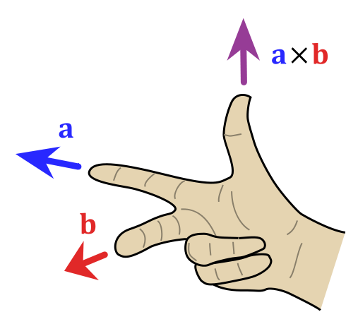
As Feynman notes, we can write this in vector form to include the directions, remembering that B is at right angles both to I as well as to r, and remembering that the order matters, of course, because of the right-hand rule for a vector cross product. 🙂
Solenoids
Coils of wire, and solenoids, pop up almost everywhere when studying electromagnetism. Indeed, transformers, inductances, electrical motors: it’s all coils. So, yes, we can’t escape them. 😦 So let’s get on with it. As you know, a solenoid is a long coil of wire wound in a tight spiral. The illustrations below show a cross-section and its magnetic field.
Now, this is probably one of Feynman’s most intuitive arguments. Read: he’s cutting an awful lot of corners here. 🙂 I’ll just copy him:
We observe experimentally that when a solenoid is very long compared with its diameter, the field outside is very small compared with the field inside. Using just that fact, together with Ampère’s law, we can find the size of the field inside. Since the field stays inside (and has zero divergence), its lines must go along parallel to the axis, as shown above. That being the case, we can use Ampère’s law with the rectangular ‘curve’ Γ shown in the figure. This loop goes the distance L inside the solenoid, where the field is, say, B0, then goes at right angles to the field, and returns along the outside, where the field is negligible. The line integral of B for this curve is just B0·L, and it must be 1/ε0c2 times the total current through Γ, which is N·I if there are N turns of the solenoid in the length L. We have:
Or, letting n be the number of turns per unit length of the solenoid (that is, n=N/L), we get:

Oh… What happens to the lines of B when they get to the end of the solenoid? Well… They just spread out in some way and return to enter the solenoid at the other end. Hmm… He’s really cutting corners here, isn’t he? But the formula is right, and I’d rather keep it short—just like he seems to want to do here. 🙂 I’ll just insert an illustration showing another right-hand rule—the right-hand rule for solenoids: if the direction of the fingers of your right hand is the direction of current, then your thumb gives the direction of the magnetic field inside.

You may wonder: does it matter where the + and − ends of the coil are? Good question because, in practice, we’ll have something that’s very tightly wound, like the coil below, so when making an actual coil (click on this link for a nice video), we’ll have several rows and so we wind from right to left and then back from left to right and so on and so on. So if we’d have two rows of wire, the two ends of the wire would come out on the same side, and that’s OK.
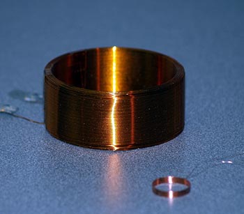
Of course, the wire needs to be insulated. What you see on the picture (and in the video) is the use of so-called magnet wire, which has a polymer film insulation. So when making the electrical connections at both ends, after winding the coil, you need to get rid of the insulation, but then it often melts just by the heat of soldering. And now that we’re talking practical stuff, let me say something about the magnetic core you see in the illustration above.
A magnetic core is a material with high magnetic permeability as compared to the surrounding air, and this high permeability will cause the magnetic field to be concentrated in the core material. Now, there’s a phenomenon that’s called hysteresis, which means that the core material will tend to retain its magnetization when the applied field is removed. This is not very desirable in many applications, such as transformers or electric engines. That’s why so-called ‘soft’ magnetic materials with low hysteresis are often preferred. The so-called soft iron is such material: it’s literally softer because of a heat treatment increasing its ductility and reducing its hardness. Of course, for permanent magnets, a so-called ‘hard’ magnetic material will be used. But here we’re getting into engineering and that’s not what I want to write about in this blog.
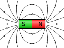
I’ll just end by noting that a magnetic field has a so-called north (N) and south (S) pole. That convention refers to the Earth’s north and south pole, of course. However, since opposite poles (north and south) attract, the North Magnetic Pole is actually the south pole of the Earth’s magnetic field, and the South is the north. 🙂 So it’s better not to think too much of the Earth’s poles when discussing the poles of a magnet. By convention, a magnet’s north pole is where the field lines of a magnet emerge, and the south pole is where they enter, as shown below.
In any case… Folks: that’s it for today. I’ll continue tomorrow. 🙂
Some content on this page was disabled on June 16, 2020 as a result of a DMCA takedown notice from The California Institute of Technology. You can learn more about the DMCA here:
https://wordpress.com/support/copyright-and-the-dmca/
Some content on this page was disabled on June 16, 2020 as a result of a DMCA takedown notice from The California Institute of Technology. You can learn more about the DMCA here:https://wordpress.com/support/copyright-and-the-dmca/
Some content on this page was disabled on June 16, 2020 as a result of a DMCA takedown notice from The California Institute of Technology. You can learn more about the DMCA here:https://wordpress.com/support/copyright-and-the-dmca/
Some content on this page was disabled on June 16, 2020 as a result of a DMCA takedown notice from The California Institute of Technology. You can learn more about the DMCA here:https://wordpress.com/support/copyright-and-the-dmca/
Some content on this page was disabled on June 16, 2020 as a result of a DMCA takedown notice from The California Institute of Technology. You can learn more about the DMCA here:https://wordpress.com/support/copyright-and-the-dmca/
Some content on this page was disabled on June 16, 2020 as a result of a DMCA takedown notice from The California Institute of Technology. You can learn more about the DMCA here:https://wordpress.com/support/copyright-and-the-dmca/
Some content on this page was disabled on June 16, 2020 as a result of a DMCA takedown notice from The California Institute of Technology. You can learn more about the DMCA here:https://wordpress.com/support/copyright-and-the-dmca/
Some content on this page was disabled on June 16, 2020 as a result of a DMCA takedown notice from The California Institute of Technology. You can learn more about the DMCA here:https://wordpress.com/support/copyright-and-the-dmca/
Some content on this page was disabled on June 16, 2020 as a result of a DMCA takedown notice from The California Institute of Technology. You can learn more about the DMCA here:https://wordpress.com/support/copyright-and-the-dmca/
Some content on this page was disabled on June 16, 2020 as a result of a DMCA takedown notice from The California Institute of Technology. You can learn more about the DMCA here:https://wordpress.com/support/copyright-and-the-dmca/
Some content on this page was disabled on June 16, 2020 as a result of a DMCA takedown notice from The California Institute of Technology. You can learn more about the DMCA here:https://wordpress.com/support/copyright-and-the-dmca/
Some content on this page was disabled on June 16, 2020 as a result of a DMCA takedown notice from The California Institute of Technology. You can learn more about the DMCA here:https://wordpress.com/support/copyright-and-the-dmca/
Some content on this page was disabled on June 20, 2020 as a result of a DMCA takedown notice from Michael A. Gottlieb, Rudolf Pfeiffer, and The California Institute of Technology. You can learn more about the DMCA here:

One thought on “Magnetostatics”