Newtonian, Lagrangian and Hamiltonian mechanics

Post scriptum (dated 16 November 2015): You’ll smile because… Yes, I am starting this post with a post scriptum, indeed. 🙂 I’ve added it, a year later or so, because, before you continue to read, you should note I am not going to explain the Hamiltonian matrix here, as it’s used in quantum physics. That’s the topic of another post, which involves far more advanced mathematical concepts. If you’re here for that, don’t read this post. Just go to my post on the matrix indeed. 🙂 But so here’s my original post. I wrote it to tie up some loose end. 🙂

As an economist, I thought I knew a thing or two about optimization. Indeed, when everything is said and done, optimization is supposed to an economist’s forte, isn’t it? 🙂 Hence, I thought I sort of understood what a Lagrangian would represent in physics, and I also thought I sort of intuitively understood why and how it could be used it to model the behavior of a dynamic system. In short, I thought that Lagrangian mechanics would be all about optimizing something subject to some constraints. Just like in economics, right?

[…] Well… When checking it out, I found that the answer is: yes, and no. And, frankly, the honest answer is more no than yes. 🙂 Economists (like me), and all social scientists (I’d think), learn only about one particular type of Lagrangian equations: the so-called Lagrange equations of the first kind. This approach models constraints as equations that are to be incorporated in an objective function (which is also referred to as a Lagrangian–and that’s where the confusion starts because it’s different from the Lagrangian that’s used in physics, which I’ll introduce below) using so-called Lagrange multipliers. If you’re an economist, you’ll surely remember it: it’s a problem written as “maximize f(x, y) subject to g(x, y) = c”, and we solve it by finding the so-called stationary points (i.e. the points for which the derivative is zero) of the (Lagrangian) objective function f(x, y) + λ[g(x, y) – c].

Now, it turns out that, in physics, they use so-called Lagrange equations of the second kind, which incorporate the constraints directly by what Wikipedia refers to as a “judicious choice of generalized coordinates.”

Generalized coordinates? Don’t worry about it: while generalized coordinates are defined formally as “parameters that describe the configuration of the system relative to some reference configuration”, they are, in practice, those coordinates that make the problem easy to solve. For example, for a particle (or point) that moves on a circle, we’d not use the Cartesian coordinates x and y but just the angle that locates the particles (or point). That simplifies matters because then we only need to find one variable. In practice, the number of parameters (i.e. the number of generalized coordinates) will be defined by the number of degrees of freedom of the system, and we know what that means: it’s the number of independent directions in which the particle (or point) can move. Now, those independent directions may or may not include the x, y and z directions (they may actually exclude one of those), and they also may or may not include rotational and/or vibratory movements. We went over that when discussing kinetic gas theory, so I won’t say more about that here.

So… OK… That was my first surprise: the physicist’s Lagrangian is different from the social scientist’s Lagrangian. 

The second surprise was that all physics textbooks seem to dislike the Lagrangian approach. Indeed, they opt for a related but different function when developing a model of a dynamic system: it’s a function referred to as the Hamiltonian. The modeling approach which uses the Hamiltonian instead of the Lagrangian is, of course, referred to as Hamiltonian mechanics. We may think the preference for the Hamiltonian approach has to do with William Rowan Hamilton being Anglo-Irish, while Joseph-Louis Lagrange (born as Giuseppe Lodovico Lagrangia) was Italian-French but… No. 🙂

And then we have good old Newtonian mechanics as well, obviously. In case you wonder what that is: it’s the modeling approach that we’ve been using all along. 🙂 But I’ll remind you of what it is in a moment: it amounts to making sense of some situation by using Newton’s laws of motion only, rather than a more sophisticated mathematical argument using more abstract concepts, such as energy, or action.

Introducing Lagrangian and Hamiltonian mechanics is quite confusing because the functions that are involved (i.e. the so-called Lagrangian and Hamiltonian functions) look very similar: we write the Lagrangian as the difference between the kinetic and potential energy of a system (L = T – V), while the Hamiltonian is the sum of both (H = T + V). Now, I could make this post very simple and just ask you to note that both approaches are basically ‘equivalent’ (in the sense that they lead to the same solutions, i.e. the same equations of motion expressed as a function of time) and that a choice between them is just a matter of preference–like choosing between an English versus a continental breakfast. 🙂 Of course, an English breakfast has usually some extra bacon, or a sausage, so you get more but… Well… Not necessarily something better. 🙂 So that would be the end of this digression then, and I should be done. However, I must assume you’re a curious person, just like me, and, hence, you’ll say that, while being ‘equivalent’, they’re obviously not the same. So how do the two approaches differ exactly?

Let’s try to get a somewhat intuitive understanding of it all by taking, once again, the example of a simple harmonic oscillator, as depicted below. It could be a mass on a spring. In fact, our example will, in fact, be that of an oscillating mass on a spring. Let’s also assume there’s no damping, because that makes the analysis soooooooo much easier.

Of course, we already know all of the relevant equations for this system just from applying Newton’s laws (so that’s Newtonian mechanics). We did that in a previous post. [I can’t remember which one, but I am sure I’ve done this already.] Hence, we don’t really need the Lagrangian or Hamiltonian. But, of course, that’s the point of this post: I want to illustrate how these other approaches to modeling a dynamic system actually work, and so it’s good we have the correct answer already so we can make sure we’re not going off track here. So… Let’s go… 🙂

I. Newtonian mechanics

Let me recapitulate the basics of a mass on a spring which, in jargon, is called a harmonic oscillator. Hooke’s law is there: the force on the mass is proportional to its distance from the zero point (i.e. the displacement), and the direction of the force is towards the zero point–not away from it, and so we have a minus sign. In short, we can write:

F = –kx (i.e. Hooke’s law)

Now, Newton‘s Law (Newton’s second law to be precise) says that F is equal to the mass times the acceleration: F = ma. So we write:

F = ma = m(d²x/dt²) = –kx

So that’s just Newton’s law combined with Hooke’s law. We know this is a differential equation for which there’s a general solution with the following form:

x(t) = A·cos(ωt + α)

If you wonder why… Well… I can’t digress on that here again: just note, from that differential equation, that we apparently need a function x(t) that yields itself when differentiated twice. So that must be some sinusoidal function, like sine or cosine, because these do that. […] OK… Sorry, but I must move on.

As for the new ‘variables’ (A, ω and α), A depends on the initial condition and is the (maximum) amplitude of the motion. We also already know from previous posts (or, more likely, because you already know a lot about physics) that A is related to the energy of the system. To be precise: the energy of the system is proportional to the square of the amplitude: E ∝ A². As for ω, the angular frequency, that’s determined by the spring itself and the oscillating mass on it: ω = (k/m)^1/2 = 2π/T = 2πf (with T the period, and f the frequency expressed in oscillations per second, as opposed to the angular frequency, which is the frequency expressed in radians per second). Finally, I should note that α is just a phase shift which depends on how we define our t = 0 point: if x(t) is zero at t = 0, then that cosine function should be zero and then α will be equal to ±π/2.

OK. That’s clear enough. What about the ‘operational currency of the universe’, i.e. the energy of the oscillator? Well… I told you already/ We don’t need the energy concept here to find the equation of motion. In fact, that’s what distinguishes this ‘Newtonian’ approach from the Lagrangian and Hamiltonian approach. But… Now that we’re at it, and we have to move to a discussion of these two animals (I mean the Lagrangian and Hamiltonian), let’s go for it.

We have kinetic versus potential energy. Kinetic energy (T) is what it always is. It depends on the velocity and the mass: K.E. = T = mv²/2 = m(dx/dt)²/2 = p²/2m. Huh? What’s this expression with p in it? […] It’s momentum: p = mv. Just check it: it’s an alternative formula for T really. Nothing more, nothing less. I am just noting it here because it will pop up again in our discussion of the Hamiltonian modeling approach. But that’s for later. Onwards!

What about potential energy (V)? We know that’s equal to V = kx²/2. And because energy is conserved, potential energy (V) and kinetic energy (T) should add up to some constant. Let’s check it: dx/dt = d[Acos(ωt + α)]/dt = –Aωsin(ωt + α). [Please do the derivation: don’t accept things at face value. :-)] Hence, T = mA²ω²sin²(ωt + α)/2 = mA²(k/m)sin²(ωt + α)/2 = kA²sin²(ωt + α)/2. Now, V is equal to V = kx²/2 = k[Acos(ωt + α)]²/2 = k[Acos(ωt + α)]²/2 = kA²cos²(ωt + α)/2. Adding both yields:

T + V = kA²sin²(ωt + α)/2 + kA²cos²(ωt + α)/2

= (1/2)kA²[sin²(ωt + α) + cos²(ωt + α)] = kA²/2.

Ouff! Glad that worked out: the total energy is, indeed, proportional to the square of the amplitude and the constant of proportionality is equal to k/2. [You should now wonder why we do not have m in this formula but, if you’d think about it, you can answer your own question: the amplitude will depend on the mass (bigger mass, smaller amplitude, and vice versa), so it’s actually in the formula already.]

The point to note is that this Hamiltonian function H = T + V is just a constant, not only for this particular case (an oscillation without damping), but in all cases where H represents the total energy of a (closed) system.

OK. That’s clear enough. How does our Lagrangian look like? That’s not a constant obviously. Just so you can visualize things, I’ve drawn the graph below:

1. The red curve represents kinetic energy (T) as a function of the displacement x: T is zero at the turning points, and reaches a maximum at the x = 0 point.
2. The blue curve is potential energy (V): unlike T, V reaches a maximum at the turning points, and is zero at the x = 0 point. In short, it’s the mirror image of the red curve.
3. The Lagrangian is the green graph: L = T – V. Hence, L reaches a minimum at the turning points, and a maximum at the x = 0 point.

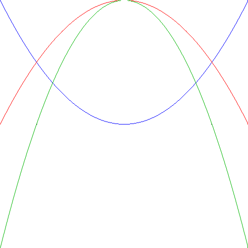
While that green function would make an economist think of some Lagrangian optimization problem, it’s worth noting we’re not doing any such thing here: we’re not interested in stationary points. We just want the equation(s) of motion. [I just thought that would be worth stating, in light of my own background and confusion in regard to it all. :-)]

OK. Now that we have an idea of what the Lagrangian and Hamiltonian functions are (it’s probably worth noting also that we do not have a ‘Newtonian function’ of some sort), let us now show how these ‘functions’ are used to solve the problem. What problem? Well… We need to find some equation for the motion, remember? [I find that, in physics, I often have to remind myself of what the problem actually is. Do you feel the same? 🙂 ] So let’s go for it.

II. Lagrangian mechanics

As this post should not turn into a chapter of some math book, I’ll just describe the how, i.e. I’ll just list the steps one should take to model and then solve the problem, and illustrate how it goes for the oscillator above. Hence, I will not try to explain why this approach gives the correct answer (i.e. the equation(s) of motion). So if you want to know why rather than how, then just check it out on the Web: there’s plenty of nice stuff on math out there.

The steps that are involved in the Lagrangian approach are the following:

1. Compute (i.e. write down) the Lagrangian function L = T – V. Hmm? How do we do that? There’s more than one way to express T and V, isn’t it? Right you are! So let me clarify: in the Lagrangian approach, we should express T as a function of velocity (v) and V as a function of position (x), so your Lagrangian should be L = L(x, v). Indeed, if you don’t pick the right variables, you’ll get nowhere. So, in our example, we have L = mv²/2 – kx²/2.
2. Compute the partial derivatives ∂L/∂x and ∂L/∂v. So… Well… OK. Got it. Now that we’ve written L using the right variables, that’s a piece of cake. In our example, we have: ∂L/∂x = – kx and ∂L/∂v = mv. Please note how we treat x and v as independent variables here. It’s obvious from the use of the symbol for partial derivatives: ∂. So we’re not taking any total differential here or so. [This is an important point, so I’d rather mention it.]
3. Write down (‘compute’ sounds awkward, doesn’t it?) Lagrange’s equation: d(∂L/∂v)/dt = ∂L/∂x. […] Yep. That’s it. Why? Well… I told you I wouldn’t tell you why. I am just showing the how here. This is Lagrange’s equation and so you should take it for granted and get on with it. 🙂 In our example: d(∂L/∂v)/dt = d(mv)/dt = –k(dx/dt) = ∂L/∂x = – kx. We can also write this as m(dv/dt) = m(d²x/dt²) = –kx.     
4. Finally, solve the resulting differential equation. […] ?! Well… Yes. […] Of course, we’ve done that already. It’s the same differential equation as the one we found in our ‘Newtonian approach’, i.e. the equation we found by combining Hooke’s and Newton’s laws. So the general solution is x(t) = Acos(ωt + α), as we already noted above.

So, yes, we’re solving the same differential equation here. So you’ll wonder what’s the difference then between Newtonian and Lagrangian mechanics? Yes, you’re right: we’re indeed solving the same second-order differential equation here. Exactly. Fortunately, I’d say, because we don’t want any other equation(s) of motion because we’re talking the same system. The point is: we got that differential equation using an entirely different procedure, which I actually didn’t explain at all: I just said to compute this and then that and… – Surprise, surprise! – we got the same differential equation in the end. 🙂 So, yes, the Newtonian and Lagrangian approach to modeling a dynamic system yield the same equations, but the Lagrangian method is much more (very much more, I should say) convenient when we’re dealing with lots of moving bits and if there’s more directions (i.e. degrees of freedom) in which they can move.

In short, Lagrange could solve a problem more rapidly than Newton with his modeling approach and so that’s why his approach won out. 🙂 In fact, you’ll usually see the spatial variables noted as q_j. In this notation, j = 1, 2,… n, and n is the number of degrees of freedom, i.e. the directions in which the various particles can move. And then, of course, you’ll usually see a second subscript i = 1, 2,… m to keep track of every q_j for each and every particle in the system, so we’ll have n×m q_ij‘s in our model and so, yes, good to stick to Lagrange in that case.

OK. You get that, I assume. Let’s move on to Hamiltonian mechanics now.

III. Hamiltonian mechanics

The steps here are the following. [Again, I am just explaining the how, not the why. You can find mathematical proofs of why this works in handbooks or, better still, on the Web.]

1. The first step is very similar as the one above. In fact, it’s exactly the same: write T and V as a function of velocity (v) and position (x) respectively and construct the Lagrangian. So, once again, we have L = L(x, v). In our example: L(x, v) = mv²/2 – kx²/2.
2. The second step, however, is different. Here, the theory becomes more abstract, as the Hamiltonian approach does not only keep track of the position but also of the momentum of the particles in a system. Position (x) and momentum (p) are so-called canonical variables in Hamiltonian mechanics, and the relation with Lagrangian mechanics is the following: p = ∂L/∂v. Huh? Yeah. Again, don’t worry about the why. Just check it for our example: ∂(mv²/2 – kx²/2)/∂v = 2mv/2 = mv. So, yes, it seems to work. Please note, once again, how we treat x and v as independent variables here, as is evident from the use of the symbol for partial derivatives. Let me get back to the lesson, however. The second step is: calculate the conjugate variables. In more familiar wording: compute the momenta.
3. The third step is: write down (or ‘build’ as you’ll see it, but I find that wording strange too) the Hamiltonian function H = T + V. We’ve got the same problem here as the one I mentioned with the Lagrangian: there’s more than one way to express T and V. Hence, we need some more guidance. Right you are! When writing your Hamiltonian, you need to make sure you express the kinetic energy as a function of the conjugate variable, i.e. as a function of momentum, rather than velocity. So we have H = H(x, p), not H = H(x, v)! In our example, we have H = T + V = p²/2m + kx²/2.
4. Finally, write and solve the following set of equations: (I) ∂H/∂p = dx/dt and (II) –∂H/∂x = dp/dt. [Note the minus sign in the second equation.] In our example: (I) p/m = dx/dt and (II) –kx = dp/dt. The first equation is actually nothing but the definition of p: p = mv, and the second equation is just Hooke’s law: F = –kx. However, from a formal-mathematical point of view, we have two first-order differential equations here (as opposed to one second-order equation when using the Lagrangian approach), which should be solved simultaneously in order to find position and momentum as a function of time, i.e. x(t) and p(t). The end result should be the same: x(t) = Acos(ωt + α) and p(t) = … Well… I’ll let you solve this: time to brush up your knowledge about differential equations. 🙂

You’ll say: what the heck? Why are you making things so complicated? Indeed, what am I doing here? Am I making things needlessly complicated?

The answer is the usual one: yes, and no. Yes. If we’d want to do stuff in the classical world only, the answer seems to be: yes! In that case, the Lagrangian approach will do and may actually seem much easier, because we don’t have a set of equations to solve. And why would we need to keep track of p(t)? We’re only interested in the equation(s) of motion, aren’t we? Well… That’s why the answer to your question is also: no! In classical mechanics, we’re usually only interested in position, but in quantum mechanics that concept of conjugate variables (like x and p indeed) becomes much more important, and we will want to find the equations for both. So… Yes. That means a set of differential equations (one for each variable (x and p) in the example above) rather than just one. In short, the real answer to your question in regard to the complexity of the Hamiltonian modeling approach is the following: because the more abstract Hamiltonian approach to mechanics is very similar to the mathematics used in quantum mechanics, we will want to study it, because a good understanding of Hamiltonian mechanics will help us to understand the math involved in quantum mechanics. And so that’s the reason why physicists prefer it to the Lagrangian approach.

[…] Really? […] Well… At least that’s what I know about it from googling stuff here and there. Of course, another reason for physicists to prefer the Hamiltonian approach may well that they think social science (like economics) isn’t real science. Hence, we – social scientists – would surely expect them to develop approaches that are much more intricate and abstract than the ones that are being used by us, wouldn’t we?

[…] And then I am sure some of it is also related to the Anglo-French thing. 🙂

Post scriptum 1 (dated 21 March 2016): I hate to write about stuff and just explain the how—rather than the why. However, in this case, the why is really rather complicated. The math behind is referred to as calculus of variations – which is a rather complicated branch of mathematics – but the physical principle behind is the Principle of Least Action. Just click the link, and you’ll see how the Master used to explain stuff like this. It’s an easy and difficult piece at the same time. Near the end, however, it becomes pretty complicated, as he applies the theory to quantum mechanics, indeed. In any case, I’ll let you judge for yourself. 🙂

Post scriptum 2 (dated 13 September 2017): I started a blog on the Exercises on Feynman’s Lectures, and the posts on the exercises on Chapter 4 have a lot more detail, and basically give you all the math you’ll ever want on this. Just click the link. However, let me warn you: the math is not easy. Not at all, really.