
Pre-script (dated 26 June 2020): This post has become less relevant (almost irrelevant, I would say) because my views on the nature of the concept of uncertainty in the context of quantum mechanics has evolved significantly as a result of my progression towards a more complete realist (classical) interpretation of quantum physics. Hence, we recommend you read our recent papers. I keep blog posts like these to see where I came from. I might review them one day, but I currently don’t have the time or energy for it. It is still interesting, though—in particular because I start by pointing out yet another error or myth in quantum mechanics that gets repeated all too often. ![]()
Original post:
One of the most confusing sentences you’ll read in an introduction to quantum mechanics – not only in those simple (math-free) popular books but also in Feynman’s Lecture introducing the topic – is that we cannot define a unique wavelength for a short wave train. In Feynman’s words: “Such a wave train does not have a definite wavelength; there is an indefiniteness in the wave number that is related to the finite length of the train, and thus there is an indefiniteness in the momentum.” (Feynman’s Lectures, Vol. I, Ch. 38, section 1).
That is not only confusing but, in some way, actually wrong. In fact, this is an oft-occurring statement which has effectively hampered my own understanding of quantum mechanics for a long time, and it was only when I had a closer look at what a Fourier analysis really is that I understood what Feynman, and others, wanted to say. In short, it’s a classic example of where a ‘simple’ account of things can lead you astray.
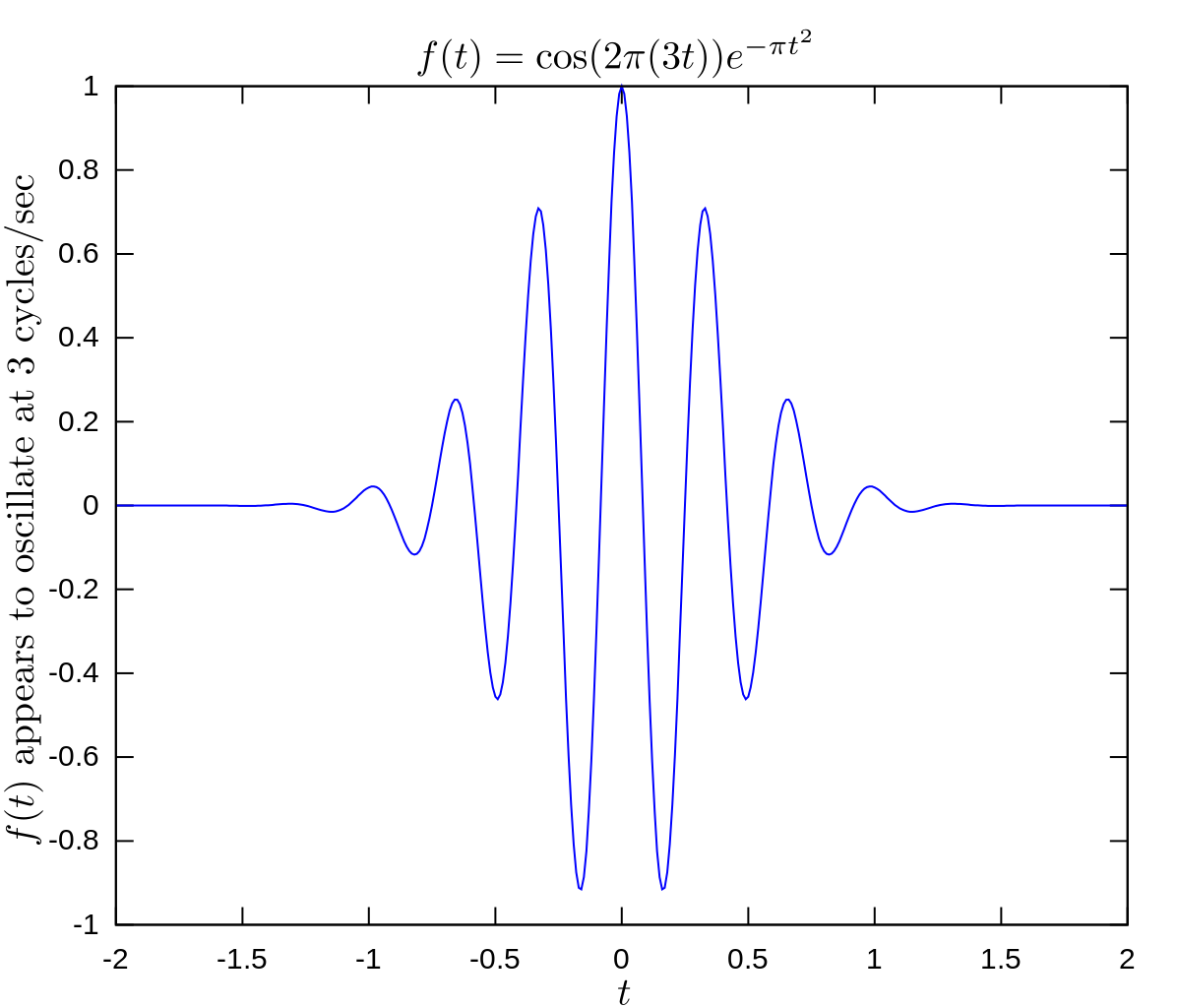
Indeed, we can all imagine a short wave train with a very definite frequency. Just take any sinusoidal function and multiply it with a so-called envelope function in order to shape it into a short pulse. Transients have that shape, and I gave an example in previous posts. Another example is given below. I copied it from the Wikipedia article on Fourier analysis: f(t) is a product of two factors:
- The first factor in the product is a cosine function: cos[2π(3t)] to be precise.
- The second factor is an exponential function: exp(–πt2).
The frequency of this ‘product function’ is quite precise: cos[2π(3t)] = cos[6πt] = cos[6π(t + 1/3)] for all values t, and so its period is equal to 1/3. [If f(x) is a function with period P, then f(ax+b), where a is a positive constant, is periodic with period P/a.] The only thing that the second factor, i.e. exp(–πt2), does is to shape this cosine function into a nice wave train, as it quickly tends to zero on both sides of the t = 0 point. So that second function is a nice simple bell curve (just plot the graph with a graph plotter) and it doesn’t change the period (or frequency) of the product. In short, the oscillation below–which we should imagine as the representation of ‘something’ traveling through space–has a very definite frequency. So what’s Feynman saying above? There’s no Δf or Δλ here, is there?
The point to note is that these Δ concepts – Δf, Δλ, and so on – actually have very precise mathematical definitions, as one would expect in physics: they usually refer to the standard deviation of the distribution of a variable around the mean.
[…] OK, you’ll say. So what?
Well… That f(t) function above can – and, more importantly, should – be written as the sum of a potentially infinite number of waves in order to make sense of the Δf and Δλ factors in those uncertainty relations. Each of these component waves has a very specific frequency indeed, and each one of them makes its own contribution to the resultant wave. Hence, there is a distribution function for these frequencies, and so that is what Δf refers to. In other words, unlike what you’d think when taking a quick look at that graph above, Δf is not zero. So what is it then?
Well… It’s tempting to get lost in the math of it all now but I don’t want this blog to be technical. The basic ideas, however, are the following. We have a real-valued function here, f(t), which is defined from –∞ to +∞, i.e. over its so-called time domain. Hence, t ranges from –∞ to +∞ (the definition of the zero point is a matter of convention only, and we can easily change the origin by adding or subtracting some constant). [Of course, we could – and, in fact, we should – also define it over a spatial domain, but we’ll keep the analysis simple by leaving out the spatial variable (x).]
Now, the so-called Fourier transform of this function will map it to its so-called frequency domain. The animation below (for which the credit must, once again, go to Wikipedia, from which I borrow most of the material here) clearly illustrates the idea. I’ll just copy the description from the same article: “In the first frames of the animation, a function f is resolved into Fourier series: a linear combination of sines and cosines (in blue). The component frequencies of these sines and cosines spread across the frequency spectrum, are represented as peaks in the frequency domain, as shown shown in the last frames of the animation). The frequency domain representation of the function,  , is the collection of these peaks at the frequencies that appear in this resolution of the function.”
[…] OK. You sort of get this (I hope). Now we should go a couple of steps further. In quantum mechanics, we’re talking not real-valued waves but complex-valued waves adding up to give us the resultant wave. Also, unlike what’s shown above, we’ll have a continuous distribution of frequencies. Hence, we’ll not have just six discrete values for the frequencies (and, hence, just six component waves), but an infinite number of them. So how does that work? Well… To do the Fourier analysis, we need to calculate the value of the following integral for each possible frequency, which I’ll denote with the Greek letter nu (ν), as we’ve used the f symbol already–not for the frequency but to denote the function itself! Let me just jot down that integral:
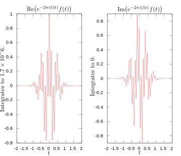
Huh? Don’t be scared now. Just try to understand what it actually represents. So just relax and take a long hard look at it. Note, first, that the integrand (i.e. the function that is to be integrated, between the integral sign and the dt, so that’s f(t)e–i2πtν) is a complex-valued function (that should be very obvious from the i in the exponent of e). Secondly, note that we need to do such integral for each value of ν. So, for each possible value of ν, we have t ranging from –∞ to +∞ in that integral. Hmm… OK. So… How does that work? Well… The illustration below shows the real and imaginary part respectively of the integrand for ν = 3. [Just in case you still don’t get it: we fix ν here (ν = 3), and calculate the value of the real and imaginary part of the integrand for each possible value of t, so t ranges from –∞ to +∞ indeed.]

So what do we see here? The first thing you should note is that the value of both the real and imaginary part of the integrand quickly tends to zero on both sides of the t = 0 point. That’s because of the shape of f(t), which does exactly the same. However, in-between those ‘zero or close-to-zero values’, the integrand does take on very specific non-zero values. As for the real part of the integrand, which is denoted by Re[e−2πi(3t)f(t)], we see that’s always positive, with a peak value equal to one at t = 0. Indeed, the real part of the integrand is always positive because f(t) and the real part of e−2πi(3t) oscillate at the same rate. Hence, when f(t) is positive, so is the real part of e−2πi(3t), and when f(t) is negative, so is the real part of e−2πi(3t). However, the story is obviously different for the imaginary part of the integrand, denoted by Im[e−2πi(3t)f(t)]. That’s because, in general, eiθ = cosθ + isinθ and the sine and cosine function are essentially the same functions except for a phase difference of π/2 (remember: sin(θ+π/2) = cosθ).
Capito? No? Hmm… Well… Try to read what I am writing above once again. Else, just give up. 🙂
I know this is getting complicated but let me try to summarize what’s going on here. The bottom line is that the integral above will yield a positive real number, 0.5 to be precise (as noted in the margin of the illustration), for the real part of the integrand, but it will give you a zero value for its imaginary part (also as noted in the margin of the illustration). [As for the math involved in calculating an integral of a complex-valued function (with a real-valued argument), just note that we should indeed just separate the real and imaginary parts and integrate separately. However, I don’t want you to get lost in the math so don’t worry about it too much. Just try to stick to the main story line here.]
In short, what we have here is a very significant contribution (the associated density is 0.5) of the frequency ν = 3.
Indeed, let’s compare it to the contribution of the wave with frequency ν = 5. For ν = 5, we get, once again, a value of zero when integrating the imaginary part of the integral above, because the positive and negative values cancel out. As for the real part, we’d think they would do the same if we look at the graph below, but they don’t: the integral does yield, in fact, a very tiny positive value: 1.7×10⁻⁶ (so we’re talking 1.7 millionths here). That means that the contribution of the component wave with frequency ν = 5 is close to nil but… Well… It’s not nil: we have some contribution here (i.e. some density in other words).
You get the idea (I hope). We can, and actually should, calculate the value of that integral for each possible value of ν. In other words, we should calculate the integral over the entire frequency domain, so that’s for ν ranging from –∞ to +∞. However, I won’t do that. 🙂 What I will do is just show you the grand general result (below), with the particular results (i.e. the values of 0.5 and 1.7×10⁻⁶ for ν = 3 and ν = 5) as a green and red dot respectively. [Note that the graph below uses the ξ symbol instead of ν: I used ν because that’s a more familiar symbol, but so it doesn’t change the analysis.]

Now, if you’re still with me – probably not 🙂 – you’ll immediately wonder why there are two big bumps instead of just one, i.e. two peaks in the density function instead of just one. [You’re used to these Gauss curves, aren’t you?] And you’ll also wonder what negative frequencies actually are: the first bump is a density function for negative frequencies indeed, and… Well… Now that you think of it: why the hell would we do such integral for negative values of ν? I won’t say too much about that: it’s a particularity which results from the fact that e2πiθ and e−2πiθ both complete a cycle per second (if θ is measured in seconds, that is) so… Well… Hmm… […] Yes. The fact of the matter is that we do have a mathematical equivalent of the bump for positive frequencies on the negative side of the frequency domain, so… Well… […] Don’t worry about it, I’d say. As mentioned above, we shouldn’t get lost in the math here. For our purpose here, which is just to illustrate what a complex Fourier transform actually is (rather than present all of the mathematical intricacies of it), we should just focus on the second bump of that density function, i.e. the density function for positive frequencies only. 🙂
So what? You’re probably tired by now, and wondering what I want to get at. Well… Nothing much. I’ve done what I wanted to do. I started with a real-valued wave train (think of a transient electric field working its way through space, for example), and I then showed how such wave train can (and should) be analyzed as consisting of an infinite number of complex-valued component waves, which each make their own contribution to the combined wave (which consists of the sum of all component waves) and, hence, can be represented by a graph like the one above, i.e. a real-valued density function around some mean, usually denoted by μ, and with some standard deviation, usually denoted by σ. So now I hope that, when you think of Δf or Δλ in the context of a so-called ‘probability wave’ (i.e. a de Broglie wave), then you’ll think of all this machinery behind.
In other words, it is not just a matter of drawing a simple figure like the one below and saying: “You see: those oscillations represent three photons being emitted one after the other by an atomic oscillator. You can see that’s quite obvious, can’t you?”
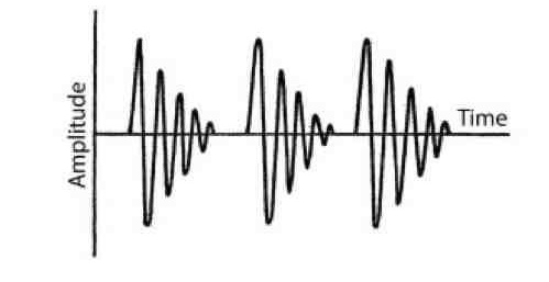
No. It is not obvious. Why not? Because anyone that’s somewhat critical will immediately say: “But how does it work really? Those wave trains seem to have a pretty definite frequency (or wavelength), even if their amplitude dies out, and, hence, the Δf factor (or Δλ factor) in that uncertainty relation must be close or, more probably, must be equal to zero. So that means we cannot say these particles are actually somewhere, because Δx must be close or equal to infinity.”
Now you know that’s a very valid remark. Because now you understand that one actually has to go through the tedious exercise of doing that Fourier transform, and so now you understand what those Δ symbols actually represent. I hope you do because of this post, and despite the fact my approach has been very superficial and intuitive. In other words, I didn’t say what physicists would probably say, and that is: “Take a good math course before you study physics!” 🙂

Thanks great ppost