Quantum math: the Hamiltonian

Pre-script (dated 26 June 2020): I have come to the conclusion one does not need all this hocus-pocus to explain quantum-mechanical systems: classical physics will do. So no use to read this. Read my papers instead. 🙂

Original post:

After all of the ‘rules’ and ‘laws’ we’ve introduced in our previous post, you might think we’re done but, of course, we aren’t. Things change. As Feynman puts it: “One convenient, delightful ‘apparatus’ to consider is merely a wait of a few minutes; During the delay, various things could be going on—external forces applied or other shenanigans—so that something is happening. At the end of the delay, the amplitude to find the thing in some state χ is no longer exactly the same as it would have been without the delay.”

In short, the picture we presented in the previous posts was a static one. Time was frozen. In reality, time passes, and so we now need to look at how amplitudes change over time. That’s where the Hamiltonian kicks in. So let’s have a look at that now.

[If you happen to understand the Hamiltonian already, you may want to have a look at how we apply it to a real situation: we’ll explain the basics involving state transitions of the ammonia molecule, which are a prerequisite to understanding how a maser works, which is not unlike a laser. But that’s for later. First we need to get the basics.]

Using Dirac’s bra-ket notation, which we introduced in the previous posts, we can write the amplitude to find a ‘thing’ – i.e. a particle, for example, or some system, of particles or other things – in some state χ at the time t = t₂, when it was in some state φ state at the time t = t₁ as follows:

Don’t be scared of this thing. If you’re unfamiliar with the notation, just check out my previous posts: we’re just replacing A by U, and the only thing that we’ve modified is that the amplitudes to go from φ to χ now depend on t₁ and t₂. Of course, we’ll describe all states in terms of base states, so we have to choose some representation and expand this expression, so we write: 

I’ve explained the point a couple of time already, but let me note it once more: in quantum physics, we always measure some (vector) quantity – like angular momentum, or spin – in some direction, let’s say the z-direction, or the x-direction, or whatever direction really. Now we can do that in classical mechanics too, of course, and then we find the component of that vector quantity (vector quantities are defined by their magnitude and, importantly, their direction). However, in classical mechanics, we know the components in the x-, y- and z-direction will unambiguously determine that vector quantity. In quantum physics, it doesn’t work that way. The magnitude is never all in one direction only, so we can always some of it in some other direction. (see my post on transformations, or on quantum math in general). So there is an ambiguity in quantum physics has no parallel in classical mechanics. So the concept of a component of a vector needs to be carefully interpreted. There’s nothing definite there, like in classical mechanics: all we have is amplitudes, and all we can do is calculate probabilities, i.e. expected values based on those amplitudes.

In any case, I can’t keep repeating this, so let me move on. In regard to that 〈 χ | U | φ 〉 expression, I should, perhaps, add a few remarks. First, why U instead of A? The answer: no special reason, but it’s true that the use of U reminds us of energy, like potential energy, for example. We might as well have used W. The point is: energy and momentum do appear in the argument of our wavefunctions, and so we might as well remind ourselves of that by choosing symbols like W or U here. Second, we may, of course, want to choose our time scale such that t₁ = 0. However, it’s fine to develop the more general case. Third, it’s probably good to remind ourselves we can think of matrices to model it all. More in particular, if we have three base states, say ‘plus‘, ‘zero, or ‘minus‘, and denoting 〈 i | φ 〉 and 〈 i | χ 〉 as C_i and D_i respectively (so 〈 χ | i 〉 = 〈 i | χ 〉* = D_i*), then we can re-write the expanded expression above as:

Fourth, you may have heard of the S-matrix, which is also known as the scattering matrix—which explains the S in front but it’s actually a more general thing. Feynman defines the S-matrix as the U(t₁, t₂) matrix for t₁ → −∞ and t₂ → +∞, so as some kind of limiting case of U. That’s true in the sense that the S-matrix is used to relate initial and final states, indeed. However, the relation between the S-matrix and the so-called evolution operators U is slightly more complex than he wants us to believe. I can’t say too much about this now, so I’ll just refer you to the Wikipedia article on that, as I have to move on.

The key to the analysis is to break things up once more. More in particular, one should appreciate that we could look at three successive points in time, t₁, t₂, t₃, and write U(t₁, t₃) as:

U(t₃, t₁) = U(t₃, t₂)·U(t₂, t₁)

It’s just like adding another apparatus in series, so it’s just like what did in our previous post, when we wrote:

So we just put a | bar between B and A and wrote it all out. That | bar is really like a factor 1 in multiplication but – let me caution you – you really need to watch the order of the various factors in your product, and read symbols in the right order, which is often from right to left, like in Hebrew or Arab, rather than from left to right. In that regard, you should note that we wrote U(t₃, t₁) rather than U(t₁, t₃): you need to keep your wits about you here! So as to make sure we can all appreciate that point, let me show you what that U(t₃, t₁) = U(t₃, t₂)·U(t₂, t₁) actually says by spelling it out if we have two base states only (like ‘up‘ or ‘down‘, which I’ll note as ‘+’ and ‘−’ again) :

So now you appreciate why we try to simplify our notation as much as we can! But let me get back to the lesson. To explain the Hamiltonian, which we need to describe how states change over time, Feynman embarks on a rather spectacular differential analysis. Now, we’ve done such exercises before, so don’t be too afraid. He substitutes t₁ for t tout court, and t₂ for t + Δt, with Δt the infinitesimal you know from Δy = (dy/dx)·Δx, with the derivative dy/dx being defined as the Δy/Δx ratio for Δx → 0. So we write U(t₂, t₁) = U(t + Δt, t). Now, we also explained the idea of an operator in our previous post. It came up when we’re being creative, and so we dropped the 〈 χ | state from the 〈 χ | A | φ〉 expression and just wrote:

If you ‘get’ that, you’ll also understand what I am writing now:

This is quite abstract, however. It is an ‘open’ equation, really: one needs to ‘complete’ it with a ‘bra’, i.e. a state like 〈 χ |, so as to give a 〈 χ | ψ〉 = 〈 χ | A | φ〉 type of amplitude that actually means something. What we’re saying is that our operator (or our ‘apparatus’ if it helps you to think that way) does not mean all that much as long as we don’t measure what comes out, so we have to choose some set of base states, i.e. a representation, which allows us to describe the final state, which we write as 〈 χ |. In fact, what we’re interested in is the following amplitudes:

So now we’re in business, really. 🙂 If we can find those amplitudes, for each of our base states i, we know what’s going on. Of course, we’ll want to express our ψ(t) state in terms of our base states too, so the expression we should be thinking of is:

Phew! That looks rather unwieldy, doesn’t it? You’re right. It does. So let’s simplify. We can do the following substitutions:

• 〈 i | ψ(t + Δt)〉 = C_i(t + Δt) or, more generally, 〈 j | ψ(t)〉 = C_j(t)
• 〈 i | U(t₂, t₁) | j〉 = U_ij(t₂, t₁) or, more specifically, 〈 i | U(t + Δt, t) | j〉 = U_ij(t + Δt, t)

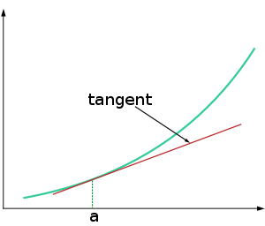
As Feynman notes, that’s how the dynamics of quantum mechanics really look like. But, of course, we do need something in terms of derivatives rather than in terms of differentials. That’s where the Δy = (dy/dx)·Δx equation comes in. The analysis looks kinda dicey because it’s like doing some kind of first-order linear approximation of things – rather than an exact kinda thing – but that’s how it is. Let me remind you of the following formula: if we write our function y as y = f(x), and we’re evaluating the function near some point a, then our Δy = (dy/dx)·Δx equation can be used to write:

y = f(x) ≈ f(a) + f'(a)·(x − a) = f(a) + (dy/dx)·Δx

To remind yourself of how this works, you can complete the drawing below with the actual y = f(x) as opposed to the f(a) + Δy approximation, remembering that the (dy/dx) derivative gives you the slope of the tangent to the curve, but it’s all kids’ stuff really and so we shouldn’t waste too much spacetime on this. 🙂

The point is: our U_ij(t + Δt, t) is a function too, not only of time, but also of i and j. It’s just a rather special function, because we know that, for Δt → 0, U_ij will be equal to 1 if i = j (in plain language: if Δt → 0 goes to zero, nothing happens and we’re just in state i), and equal to 0 if i = j. That’s just as per the definition of our base states. Indeed, remember the first ‘rule’ of quantum math:

〈 i | j〉 = 〈 j | i〉 = δ_ij, with δ_ij = δ_ji is equal to 1 if i = j, and zero if i ≠ j

So we can write our f(x) ≈ f(a) + (dy/dx)·Δx expression for U_ij as:

So K_ij is also some kind of derivative and the Kronecker delta, i.e. δ_ij, serves as the reference point around which we’re evaluating U_ij. However, that’s about as far as the comparison goes. We need to remind ourselves that we’re talking complex-valued amplitudes here. In that regard, it’s probably also good to remind ourselves once more that we need to watch the order of stuff: U_ij = 〈 i | U | j〉, so that’s the amplitude to go from base state j to base state i, rather than the other way around. Of course, we have the 〈 χ | φ 〉 = 〈 φ | χ 〉* rule, but we still need to see how that plays out with an expression like 〈 i | U(t + Δt, t) | j〉. So, in short, we should be careful here! 

Having said that, we can actually play a bit with that expression, and so that’s what we’re going to do now. The first thing we’ll do is to write K_ij as a function of time indeed:

K_ij = K_ij(t)

So we don’t have that Δt in the argument. It’s just like dy/dx = f'(x): a derivative is a derivative—a function which we derive from some other function. However, we’ll do something weird now: just like any function, we can multiply or divide it by some constant, so we can write something like G(x) = c·F(x), which is equivalent to saying that F(x) = G(x)/c. I know that sound silly but it is how is, and we can also do it with complex-valued functions: we can define some other function by multiplying or dividing by some complex-valued constant, like a + b·i, or ξ or whatever other constant. Just note we’re no longer talking the base state i but the imaginary unit i. So it’s all done so as to confuse you even more. 🙂

So let’s take −i/ħ as our constant and re-write our K_ij(t) function as −i/ħ times some other function, which we’ll denote by H_ij(t), so K_ij(t) = –(i/ħ)·H_ij(t). You guess it, of course: H_ij(t) is the infamous Hamiltonian, and it’s written the way it’s written both for historical as well as for practical reasons, which you’ll soon discover. Of course, we’re talking one coefficient only and we’ll have nine if we have three base states i and j, or four if we have only two. So we’ve got a n-by-n matrix once more. As for its name… Well… As Feynman notes: “How Hamilton, who worked in the 1830s, got his name on a quantum mechanical matrix is a tale of history. It would be much better called the energy matrix, for reasons that will become apparent as we work with it.”

OK. So we’ll just have to acknowledge that and move on. Our U_ij(t + Δt, t) = δ_ij + K_ij(t)·Δt expression becomes:

 U_ij(t + Δt, t) = δ_ij –(i/ħ)·H_ij(t)·Δt

[Isn’t it great you actually start to understand those Chinese-looking formulas? :-)] We’re not there yet, however. In fact, we’ve still got quite a bit of ground to cover. We now need to take that other monster:

So let’s substitute now, so we get:

We can get this in the form we want to get – so that’s the form you’ll find in textbooks 🙂 – by noting that the ∑δ_ij·C_j(t) sum, taking over all j is, quite simply, equal to C_i(t). [Think about the indexes here: we’re looking at some i, and so it’s only the j that’s taking on whatever value it can possibly have.] So we can move that to the other side, which gives us C_i(t + Δt) – C_i(t). We can then divide both sides of our expression by Δt, which gives us an expression like [f(x + Δx) – f(x)]/Δx = Δy//Δx, which is actually the definition of the derivative for Δx going to zero. Now, that allows us to re-write the whole thing in terms of a proper derivative, rather than having to work with this rather unwieldy differential stuff. So, if we substitute [C_i(t + Δt) – C_i(t)]/Δx for d[C_i(t)]/dt, and then also move –(i/ħ) to the left-hand side, remembering that 1/i = –i (and, hence, [–(i/ħ)]⁻¹ = i/ħ), we get the formula in the shape we wanted it in:

Done ! Of course, this is a set of differential equations and… Well… Yes. Yet another set of differential equations. 🙂 It seems like we can’t solve anything without involving differential equations in physics, isn’t it? But… Well… I guess that’s the way it is. So, before we turn to some example, let’s note a few things.

First, we know that a particle, or a system, must be in some state at any point of time. That’s equivalent to stating that the sum of the probabilities |C_i(t)|² = |〈 i | ψ(t)〉|² is some constant. In fact, we’d like to say it’s equal to one, but then we haven’t normalized anything here. You can fiddle with the formulas but it’s probably easier to just acknowledge that, if we’d measure anything – think of the angular momentum along the z-direction, or some other direction, if you’d want an example – then we’ll find it’s either ‘up’ or ‘down’ for a spin-1/2 particle, or ‘plus’, ‘zero’, or ‘minus’ for a spin-1 particle.

Now, we know that the complex conjugate of a sum is equal to the sum of the complex conjugates: [∑ z_i ]* = ∑ z_i*, and that the complex conjugate of a product is the product of the complex conjugates, so we have [∑ z_iz_j ]* = ∑ z_i*z_j*. Now, some fiddling with the formulas above should allow you to prove that H_ij = H_ij*, and the associated matrix is usually referred to as the Hermitian or conjugate transpose. If if the original Hamiltonian matrix is denoted as H, then its conjugate transpose will be denoted by H*, H^† or even H^H (so the H in the superscript stands for Hermitian, instead of Hamiltonean). So… Yes. There’s competing notations around. 🙂

The simplest situation, of course, is when the Hamiltonian do not depend on time. In that case, we’re back in the static case, and all H_ij coefficients are just constants. For a system with two base states, we’d have the following set of equations:

This set of two equations can be easily solved by remembering the solution for one equation only. Indeed, if we assume there’s only base state – which is like saying: the particle is at rest somewhere (yes: it’s that stupid!) – our set of equations reduces to only one:

This is a differential equation which is easily solved to give:

[As for being ‘easily solved’, just remember the exponential function is its own derivative and, therefore, d[a·e^{–(i/ħ)H_ijt}]/dt = a·d[e^{–(i/ħ)H_ijt}]/dt = –a·(i/ħ)·H_ij·e^{–(i/ħ)H_ijt}, which gives you the differential equation, so… Well… That’s the solution.]

This should, of course, remind you of the equation that inspired Louis de Broglie to write down his now famous matter-wave equation (see my post on the basics of quantum math):

a·e^−i·θ = e^{−i·(ω·t − k ∙x)} = a·e^{−(i/ħ)·(E·t − p∙x)}

Indeed, if we look at the temporal variation of this function only – so we don’t consider the space variable x – then this equation reduces to a·e^{–(i/ħ)·(E·t)}, and so find that our Hamiltonian coefficient H₁₁ is equal to the energy of our particle, so we write: H₁₁ = E, which, of course, explains why Feynman thinks the Hamiltonian matrix should be referred to as the energy matrix. As he puts it: “The Hamiltonian is the generalization of the energy for more complex situations.”

Now, I’ll conclude this post by giving you the answer to Feynman’s remark on why the Irish 19th century mathematician William Rowan Hamilton should be associated with the Hamiltonian. The truth is: the term ‘Hamiltonian matrix’ may also refer to a more general notion. Let me copy Wikipedia here: “In mathematics, a Hamiltonian matrix is a 2n-by-2n matrix A such that JA is symmetric, where J is the skew-symmetric matrix

and I_n is the n-by-n identity matrix. In other words, A is Hamiltonian if and only if (JA)^T = JA where ()^T denotes the transpose. So… That’s the answer. 🙂 And there’s another reason too: Hamilton invented the quaternions and… Well… I’ll leave it to you to check out what these have got to do with quantum physics. 🙂

[…] Oh ! And what about the maser example? Well… I am a bit tired now, so I’ll just refer you to Feynman’s exposé on it. It’s not that difficult if you understood all of the above. In fact, it’s actually quite straightforward, and so I really recommend you work your way through the example, as it will give you a much better ‘feel’ for the quantum-mechanical framework we’ve developed so far. In fact, walking through the whole thing is like a kind of ‘reward’ for having worked so hard on the more abstract stuff in this and my previous posts. So… Yes. Just go for it! 🙂 [And, just in case you don’t want to go for it, I did write a little introduction to in the following post. :-)]

Some content on this page was disabled on June 16, 2020 as a result of a DMCA takedown notice from The California Institute of Technology. You can learn more about the DMCA here:

https://en.support.wordpress.com/copyright-and-the-dmca/
Some content on this page was disabled on June 16, 2020 as a result of a DMCA takedown notice from The California Institute of Technology. You can learn more about the DMCA here:

https://en.support.wordpress.com/copyright-and-the-dmca/
Some content on this page was disabled on June 16, 2020 as a result of a DMCA takedown notice from The California Institute of Technology. You can learn more about the DMCA here:

https://en.support.wordpress.com/copyright-and-the-dmca/
Some content on this page was disabled on June 16, 2020 as a result of a DMCA takedown notice from The California Institute of Technology. You can learn more about the DMCA here:

https://en.support.wordpress.com/copyright-and-the-dmca/
Some content on this page was disabled on June 16, 2020 as a result of a DMCA takedown notice from The California Institute of Technology. You can learn more about the DMCA here:

https://en.support.wordpress.com/copyright-and-the-dmca/
Some content on this page was disabled on June 16, 2020 as a result of a DMCA takedown notice from The California Institute of Technology. You can learn more about the DMCA here:

https://en.support.wordpress.com/copyright-and-the-dmca/
Some content on this page was disabled on June 16, 2020 as a result of a DMCA takedown notice from The California Institute of Technology. You can learn more about the DMCA here:

https://en.support.wordpress.com/copyright-and-the-dmca/
Some content on this page was disabled on June 16, 2020 as a result of a DMCA takedown notice from The California Institute of Technology. You can learn more about the DMCA here:

https://en.support.wordpress.com/copyright-and-the-dmca/
Some content on this page was disabled on June 16, 2020 as a result of a DMCA takedown notice from The California Institute of Technology. You can learn more about the DMCA here:

https://en.support.wordpress.com/copyright-and-the-dmca/
Some content on this page was disabled on June 17, 2020 as a result of a DMCA takedown notice from Michael A. Gottlieb, Rudolf Pfeiffer, and The California Institute of Technology. You can learn more about the DMCA here:

https://en.support.wordpress.com/copyright-and-the-dmca/
Some content on this page was disabled on June 17, 2020 as a result of a DMCA takedown notice from Michael A. Gottlieb, Rudolf Pfeiffer, and The California Institute of Technology. You can learn more about the DMCA here:

https://en.support.wordpress.com/copyright-and-the-dmca/