
Pre-scriptum (dated 26 June 2020): This post – part of a series of rather simple posts on elementary math and physics – has suffered only a little bit from the attack by the dark force—which is good because I still like it. A few illustrations were removed because of perceived ‘unfair use’, but you will be able to google equivalent stuff. While my views on the true nature of light, matter and the force or forces that act on them have evolved significantly as part of my explorations of a more realist (classical) explanation of quantum mechanics, I think most (if not all) of the analysis in this post remains valid and fun to read. In fact, I would dare to say the whole Universe is all about resonance!
Original post:
One of the most common behaviors of physical systems is the phenomenon of resonance: a body (not only a tuning fork but any body really, such as a body of water, such as the ocean for example) or a system (e.g. an electric circuit) will have a so-called natural frequency, and an external driving force will cause it to oscillate. How it will behave, then, can be modeled using a simple differential equation, and the so-called resonance curve will usually look the same, regardless of what we are looking at. Besides the standard example of an electric circuit consisting of (i) a capacitor, (ii) a resistor and (iii) an inductor, Feynman also gives the following non-standard examples:
1. When the Earth’s atmosphere was disturbed as a result of the Krakatoa volcano explosion in 1883, it resonated at its own natural frequency, and its period was measured to be 10 hours and 20 minutes.
[In case you wonder how one can measure that, an explosion such as that one creates all kinds of waves, but the so-called infrasonic waves are the one we are talking about here. They circled the globe at least seven times, shattering windows hundreds of miles away. They did not only shatter windows in a radius , but they were also recorded worldwide. That’s how they could be measured a second, third, etc time. How? There was no wind or so, but the infrasonic waves (i.e. ‘sounds’ beneath the lowest limits of human hearing (about 16 or 17 Hz), down to 0.001 Hz) of such oscillation cause minute changes in the atmospheric pressure which can be measured by microbarometers. So the ‘ringing’ of the atmosphere was measurable indeed. A nice article on infrasound waves is journal.borderlands.com/1997/infrasound. Of course, the surface of the Earth was ‘ringing’ as well, and such seismic shocks then produce tsunami waves, which can also be analyzed in terms of natural frequencies.]
2. Crystals can be made to oscillate in response to a changing external electric field, and this crystal resonance phenomenon is used in quartz clocks: the quartz crystal resonator in a basic quartz wristwatch is usually in the shape of a very small tuner fork. Literally: there’s a tiny tuning fork in your wristwatch, made of quartz, that has been laser-trimmed to vibrate at exactly 32,768 Hz, i.e. 215 cycles per second.
3. Some quantum-mechanical phenomena can be analyzed in terms of resonance as well, but then it’s the energy of the interfering particles that assumes the role of the frequency of the external driving force when analyzing the response of the system. Feynman gives the example of gamma radiation from lithium as a function of the energy of protons bombarding the lithium nuclei to provoke the reaction. Indeed, when graphing the intensity of the gamma radiation emitted as a function of the energy, one also gets a resonance curve, as shown below. [Don’t you just love the fact it’s so old? A Physical Review article of 1948! There’s older stuff as well, because this journal actually started in 1893.]

However, let us analyze the phenomenon first in its most classical appearance: an oscillating spring.
Basics
We’ve seen the equation for an oscillating spring before. From a math point of view, it’s a differential equation (because one of the terms is a derivative of the dependent variable x) of the second order (because the derivative involved is of the second order):
m(d2x/dt2) = –kx
What’s written here is simply Newton’s Law: the force is –kx (the minus sign is there because the force is directed opposite to the displacement from the equilibrium position), and the force has to equal the oscillating mass on the spring times its acceleration: F = ma.
Now, this can be written as d2x/dt2 = –(k/m)x = –ω02x with ω02 = k/m. This ω0 symbol uses the Greek omega once again, which we used for the angular velocity of a rotating body. While we do not have anything that’s rotating here, ω0 is still an angular velocity or, to be more precise, it’s an angular frequency. Indeed, the solution to the differential equation above is
x = x0cos(ω0t + Δ)
The x0 factor is the maximum amplitude and that’s, quite simply, determined by how far we pulled or pushed the spring when we started the motion. Now, ω0t + Δ = θ is referred to as the phase of the motion, and it’s easy to see that ω0 is an angular frequency indeed, because ω0 equals the time derivative dθ/dt. Hence, ω0 is the phase change, measured in radians, per second, and that’s the definition of angular frequency or angular velocity. Finally, we have Δ. That’s just a phase shift, and it basically depends on our t = 0 point.
Something on the math
I’ll do a separate post on the math that’s associated with this (second-order differential equations) but, in this case, we can solve the equation in a simple and intuitive way. Look at it: d2x/dt2 = –ω02x. It’s obvious that x has to be a function that comes back to itself after two derivations, but with a minus sign in front, and then we also have that coefficient –ω02. Hmm… What can we think of? An exponential function comes back to itself, and if there’s a coefficient in the exponent, then it will end up as a coefficient in front too: d(eat)/dt = aeat and, hence, d2(eat)/dt2 = a2eat. Waw ! That’s close. In fact, that’s the same equation as the one above, except for the minus sign.
In fact, if you’d quickly look at Paul’s Online Math Notes, you’ll see that we can indeed get the general solution for such second-order differential equation (to be precise: it’s a so-called linear and homogeneous second-order DE with constant coefficients) using that remarkable property of exponentials indeed. However, because of the minus sign, our solution for the equation above will involve complex exponentials, and so we’ll get a general function in a complex variable. However, we’ll then impose that our solution has to be real only and, hence, we’ll take a subset of our more general solution. However, don’t worry about that here now. There’s an easier way.
Apart from the exponential function, there are two other functions that come back to themselves after two derivatives: the sine and cosine functions. Indeed, d2cos(t)/dt2 = –cos(t) and d2sin(t)/dt2 = –sin(t). In fact, the sine and cosine function are obviously the same except for a phase shift equal π/2: cos(t) = sin(t + π/2), so we can choose either. Let’s work with the cosine as for now (we can always convert it to a sine function using that cos(t) = sin(t + π/2) identity). The nice thing about the cosine (and sine) function is that we do get that minus sign when deriving it two times, and we also get that coefficient in front. Indeed: d2cos(ω0t)/dt2 = –ω02cos(ω0t). In short, cos(ω0t) is the right function. The only thing we need to add is that x0 and Δ, i.e. the amplitude and some phase shift but, as mentioned above, it is easy to understand these will depend on the initial conditions (i.e. the value of x at point t = 0 and the initial pull or push on the spring). In short, x = x0cos(ω0t + Δ) is the complete general solution of the simple (differential) equation we started with (i.e. m(d2x/dt2) = –kx).
Introducing a driving force
Now, most real-life oscillating systems will be driven by an external force, permanently or just for a short while, and they will also lose some of their energy in a so-called dissipative process: friction or, in an electric circuit, electrical resistance will cause the oscillation to slowly lose amplitude, thereby damping it.
Let’s look at the friction coefficient first. The friction will often be proportional to the speed with which the object moves. Indeed, in the case of a mass on a spring, the drag (i.e. the force that acts on a body as it travels through air or a fluid) is dependent on a lot of things: first and foremost, there’s the fluid itself (e.g. a thick liquid will create more drag than water), and then there’s also the size, shape and velocity of the object. I am following the treatment you’ll find in most textbooks here and so that includes an assumption that the resistance force is proportional to the velocity: Ff = –cv = –c(dx/dt). Furthermore, the constant of proportionality c will usually be written as a product of the mass and some other coefficient γ, so we have Ff = –cv = –mγ(dx/dt). That makes sense because we can look at γ = c/m as the friction per unit of mass.
That being said, the simplification as a whole (i.e. the assumption of proportionality with speed) is rather strange in light of the fact that drag forces are actually proportional to the square of the velocity. If you look it up, you’ll find a formula resembling FD = ρCDAv2/2, with ρ the fluid density, CD the drag coefficient of drag (determined by the shape of the object and a so-called Reynolds number, which is determined from experiments), and A the cross-section area. It’s also rather strange to relate drag to mass by writing c as c = mγ because drag has nothing to do with mass. What about dry friction? So that would be kinetic friction between two surfaces, like when the mass is sliding on a surface? Well… In that case, mass would play a role but velocity wouldn’t, because kinetic friction is independent of the sliding velocity.
So why do physicists use this simplification? One reason is that it works for electric circuits: the equivalent of the velocity in electrical resonance is the current I = dq/dt, so that’s the time derivative of the charge on the capacitor. Now, I is proportional to the voltage difference V, and the proportionality coefficient is the resistance R, so we have V = RI = R(dq/dt). So, in short, the resistance curve we’re actually going to derive below is one for electric circuits. The other reason is that this assumption makes it easier to solve the differential equation that’s involved: it makes for a linear differential equation indeed. In fact, that’s the main reason. After all, professors are professors and so they have to give their students stuff that’s not too difficult to solve. In any case, let’s not be bothered too much and so we’ll just go along with it.
Modeling the driving force is easy: we’ll just assume it’s a sinusoidal force with angular frequency ω (and ω is, obviously, more likely than not somewhat different than the natural frequency ω0). If F is sinusoidal force, we can write it as F = F0cos(ωt + Δ). [So we also assume there is some phase shift Δ.] So now we can write the full equation for our oscillating spring as:
m(d2x/dt2) + γm(dx/dt) + kx = F ⇔ (d2x/dt2)+ γ(dx/dt) + ω02x = F
How do we solve something like that for x? Well, it’s a differential equation once again. In fact, it’s, once again, a linear differential equation with constant coefficients, and so there’s a general solution method for that. As I mentioned above, that general solution method will involve exponentials and, in general, complex exponentials. I won’t walk you through that. Indeed, I’ll just write the solution because this is not an exercise in solving differential equations. I just want you to understand the solution:
x = ρF0cos(ωt + Δ + θ)
ρ in this equation has nothing to do with some density or so. It’s a factor which depends on m, ω and ω0, in a fairly complicated way in fact:
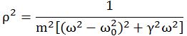
As we can see from the equation above, the (maximum) amplitude of the oscillation is equal to ρF0. So we have the magnitude of the force F here multiplied by ρ. Hence, ρ is a magnification factor which, multiplied with F0, gives us the ‘amount’ of oscillation.
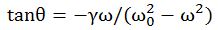
As for the θ in the equation above, we’re using this Greek letter (theta) not to refer to the phase, as we usually do, because the phase here is the whole ωt + Δ + θ expression, not just theta! The theta (θ) here is a phase shift as compared to the original force phase ωt + Δ, and θ also depends on ω and ω0. Again, I won’t show how we derived this solution but just accept it as for now:
These three equations, taken together, should allow you to understand what’s going on really. We’ve got an oscillation x = ρF0cos(ωt + Δ + θ), so that’s an equation with this amplification or magnification factor ρ and some phase shift θ. Both depend on the difference between ω0 and ω, and the two graphs below show how exactly.
The first graph shows the resonance phenomenon and, hence, it’s what’s referred to as the resonance curve: if the difference between ω0 and ω is small, we get an enormous amplification effect. It would actually go to infinity if it weren’t for the frictional force (but, of course, if the frictional force was not there, the spring would just break as the oscillation builds up and the swings get bigger and bigger).
The second graph shows the phase shift θ. It is interesting to note that the lag θ is equal –π/2 when ω0 is equal to ω, but I’ll let you figure out why this makes sense. [It’s got something to do with that cos(t) = sin(t + π/2) identity, so it’s nothing ‘deep’ really.]
I guess I should, perhaps, also write something about the energy that gets stored in an oscillator like this because, in that resonance curve above, we actually have ρ squared on the vertical axis, and that’s because energy is proportional to the square of the amplitude: E ∝ A2. I should also explain a concept that’s closely related to energy: the so-called Q of an oscillator. It’s an interesting topic, if only because it helps us to understand why, for instance, the waves of the sea are such tremendous stores of energy! Furthermore, I should also write something about transients, i.e. oscillations that dampen because the driving force was turned off so to say. However, I’ll leave that for you to look it up if you’re interested in this topic. Here, I just wanted to present the essentials.
[…] Hey ! I managed to keep this post quite short for a change. Isn’t that good? 🙂
Some content on this page was disabled on June 16, 2020 as a result of a DMCA takedown notice from The California Institute of Technology. You can learn more about the DMCA here:
https://wordpress.com/support/copyright-and-the-dmca/
Some content on this page was disabled on June 16, 2020 as a result of a DMCA takedown notice from The California Institute of Technology. You can learn more about the DMCA here:https://wordpress.com/support/copyright-and-the-dmca/
Some content on this page was disabled on June 16, 2020 as a result of a DMCA takedown notice from The California Institute of Technology. You can learn more about the DMCA here:
