Loose ends: on energy of radiation and polarized light

Pre-scriptum (dated 26 June 2020): Some of the relevant illustrations in this post were removed as a result of an attack by the dark force. Too bad, because I liked this post. In any case, despite the removal of the illustrations, you should be able to reconstruct the main story line.

Original post:

I said I would move on to another topic, but let me wrap up some loose ends in this post. It will say a few things about the energy of a field; then it will analyze these electron oscillators in some more detail; and, finally, I’ll say a few words about polarized light.

The energy of a field

You may or may not remember, from our discussions on oscillators and energy, that the total energy in a linear oscillator is a constant sum of two variables: the kinetic energy mv²/2 and the potential energy (i.e. the energy stored in the spring as it expands and contracts) kx²/2 (remember that the force is -kx). So the kinetic energy is proportional to the square of the velocity, and the potential energy to the square of the displacement. Now, from the general solution that we had obtained for a linear oscillator – damped or not – we know that the displacement x, its velocity dx/dt, and even its acceleration are all proportional to the magnitude of the field – with different factors of proportionality of course. Indeed, we have x = q_eE₀e^iωt/m(ω₀²–ω²), and so every time we take a derivative, we’ll be bring a iω factor down (and so we’ll have another factor of proportionality), but the E₀ factor is still the same, and a factor of proportionality multiplied with some constant is still a factor of proportionality. Hence, the energy should be proportional to the square of the amplitude of the motion E₀. What more can we say about it?

The first thing to note is that, for a field emanating from a point source, the magnitude of the field vector E will vary inversely with r. That’s clear from our formula for radiation:

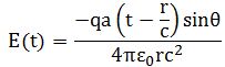
Hence, the energy that the source can deliver will vary inversely as the square of the distance. That implies that the energy we can take out of a wave, within a given conical angle, will always be the same, not matter how far away we are. What we have is an energy flux spreading over a greater and greater effective area. That’s what’s illustrated below: the energy flowing within the cone OABCD is independent of the distance r at which it is measured.

However, these considerations do not answer the question: what is that factor of proportionality? What’s its value? What does it depend on?

We know that our formula for radiation is an approximate formula, but it’s accurate for what is called the “wave zone”, i.e. for all of space as soon as we are more than a few wavelengths away from the source. Likewise, Feynman derives an approximate formula only for the energy carried by a wave using the same framework that was used to derive the dispersion relation. It’s a bit boring – and you may just want to go to the final result – but, well… It’s kind of illustrative of how physics analyzes physical situations and derives approximate formulas to explain them.

Let’s look at that framework again: we had a wave coming in, and then a wave being transmitted. In-between, the plate absorbed some of the energy, i.e. there was some damping. The situation is shown below, and the exact formulas were derived in the previous post.

Now, we can write the following energy equation for a unit area:

Energy in per second = energy out per second + work done per second

That’s simple, you’ll say. Yes, but let’s see where we get with this. For the energy that’s going in (per second), we can write that as α〈E_s²〉, so that’s the averaged square of the amplitude of the electric field emanating from the source multiplied by a factor α. What factor α? Well… That’s exactly what we’re trying to find out: be patient.

For the energy that’s going out per second, we have α〈E_s² + E_a²〉. Why the same α? Well… The transmitted wave is traveling through the same medium as the incoming wave (air, most likely), so it should be the same factor of proportionality. Now, α〈E_s² + E_a²〉 = α[〈E_s²〉 + 2〈E_s〉〈E_a〉 + 〈E_a²〉]. However, we know that we’re looking at a very thin plate here only, and so the amplitude E_a must be small as compared to E_a. So we can leave its averaged square 〈E_a²〉 value out. Indeed, as mentioned above, we’re looking at an approximation here: any term that’s proportional with NΔz, we’ll leave in (and so we’ll leave 〈E_s〉〈E_a〉 in), but terms that are proportional to (NΔz)² or a higher power can be left out. [That’s, in fact, also the reason why we don’t bother to analyze the reflected wave.]

So we now have the last term: the work done per second in the plate. Work done is force times distance, and so the work done per second (i.e. the power being delivered) is the force times the velocity. [In fact, we should do a dot product but the force and the velocity point are along the same direction – except for a possible minus sign – and so that’s alright.] So, for each electron oscillator, the work done per second will be 〈q_eE_sv〉 and, hence, for a unit area, we’ll have NΔzq_e〈E_sv〉. So our energy equation becomes:

α〈E_s²〉 = α〈E_s²〉 + 2α〈E_s〉〈E_a〉 + NΔzq_e〈E_sv〉

⇔ –2α〈E_s〉〈E_a〉 = NΔzq_e〈E_sv〉

Now, we had a formula for E_a (we didn’t do the derivation of this one though: just accept it):

We can substitute this in the energy equation, noting that the average of E_a is not dependent from time. So the left-hand side of our energy equation becomes:

 

However, E_s(at z) is E_s(at atoms) retarded by z/c, so we can insert the same argument. But then, now that we’ve made sure that we got the same argument for E_s and v, we know that such average is independent of time and, hence, it will be equal to the 〈E_sv〉 factor on the right-hand side of our energy equation, which means this factor can be scrapped. The NΔzq_e (and that 2 in the numerator and denominator) can be scrapped as well, of course. We then get the remarkably simple result that

α = ε₀c

Hence, the energy carried in an electric wave per unit area and per unit time, which is also referred to as the intensity of the wave, equals:

〈S〉 = ε₀c〈E〉

The rate of radiation of energy

Plugging our formula for radiation above into this formula, we get an expression for the power per square meter radiated in the direction q:

In this formula, a’ is, of course, the retarded acceleration, i.e. the value of a at point t – r/c. The formula makes it clear that the power varies inversely as the square of the distance, as it should, from what we wrote above. I’ll spare you the derivation (you’ve had enough of these derivations,  I am sure), but we can use this formula to calculate the total energy radiated in all directions, by integrating the formula over all directions. We get the following general formula:

This formula is no longer dependent on the distance r – which is also in line with what we said above: in a given cone, the energy flux is the same. In this case, the ‘cone’ is actually a sphere around the oscillating charge, as illustrated below.

Now, we usually assume we have a nice sinusoidal function for the displacement of the charge and, hence, for the acceleration, so we’ll often assume that the acceleration a equals a = –ω²x₀e^iωt. In that case, we can average over a cycle (note that the average of a cosine is one-half) and we get:

Now, historically, physicists used a value written as e², not to be confused with the transcendental number e, equal to e² = q_e²/4πe₀, which – when inserted above – yields the older form of the formula above:

P = 2e²a²/3c³

In fact, we actually worked with that e² factor already, when we were talking about potential energy and calculated the potential energy between a proton and an electron at distance r: that potential energy was equal to e²/r but that was a while ago indeed – and so you’ll probably not remember.

Atomic oscillators

Now, I can imagine you’ve had enough of all these formulas. So let me conclude by giving some actual numbers and values for things. Let’s look at these atomic oscillators and put some values in indeed. Let’s start with calculating the Q of an atomic oscillator.

You’ll remember what the Q of an oscillator is: it is a measure of the ‘quality’ (that’s what the Q stands for really) of a particular oscillator. A high Q implies that, if we ‘hit’ the oscillator, it will ‘ring’ for many cycles, so its decay time will be quite long. It also means that the peak width of its ‘frequency response’ will be quite tall. Huh? The illustrations below will refresh your memory.

The first one (below) gives a very general form for a typical resonance: we have a fixed frequency f₀ (which defines the period T, and vice versa), and so this oscillator ‘rings’ indeed, and slowly dies out. An associated concept is the decay time (τ) of an oscillation: that’s the time it takes for the amplitude of the oscillation to fall by a factor 1/e = 1/2.7182… ≈ 36.8% of the original value.

The second illustration (below) gives the frequency response curve. That assumes there is a continuous driving force, and we know that the oscillator will react to that driving force by oscillating – after an initial transient – at the same frequency driving force, but its amplitude will be determined by (i) the difference between the frequency of the driving force and the oscillator’s natural frequency (f₀) as well as (ii) the damping factor. We will not prove it here, but the ‘peak height’ is equal to the low-frequency response (C) multiplied by the Q of the system, and the peak width is f₀ divided by Q.

But what is the Q for an atomic oscillator? Well… The Q of any system is the total energy content of the oscillator and the work done (or the energy loss) per radian. [If we define it per cycle, then we need to throw an additional 2π factor in – that’s just how the Q has been defined !] So we write:

Q = W/(dW/dΦ)

Now, dW/dΦ = (dW/dt)/(dΦ/dt) = (dW/dt)/ω, so Q = ωW/(dW/dt), which can be re-written as the first-order differential equation dW/dt = -(ω/Q)W. Now, that equation has the general solution

W = W₀e^–ωt/Q, with W₀ the initial energy.

Using our energy equation – and assuming that our atomic oscillators are radiating at some natural (angular) frequency ω₀, which we’ll relate to the wavelength λ = 2πc/ω₀ – we can calculate the Q. But what do we use for W₀? Well… The kinetic energy of the oscillator is mv²/2. Assuming the displacement x has that nice sinusoidal shape, we get mω²x₀²/4 for the mean kinetic energy, which we have to double to get the total energy (remember that, on average, the total energy of an oscillator is half kinetic, and half potential), so then we get W = mω²x₀²/2. Using m_e (the electron mass) for m, we can then plug it all in, divide and cancel what we need to divide and cancel, and we get the grand result:

 Q = Q = ωW/(dW/dt) = 3λm_ec²/4πe² or 1/Q =  4πe²/3λm_ec²

The second form is preferred because it allows substituting e²/m_ec² for yet another ‘historical’ constant, referred to as the classical electron radius r₀ = e²/m_ec² = 2.82×10^–15 m. However, that’s yet another diversion, and I’ll try to spare you here. Indeed, we’re almost done so let’s sprint to the finish.

So all we need now is a value for λ. Well… Let’s just take one: a sodium atom emits light with a wavelength of approximately 600 nanometer. Yes, that’s the yellow-orange light emitted by low-pressure sodium-vapor lamps used for street lighting. So that’s a typical wavelength and we get a Q equal to

Q = 3λ/4πr₀ ≈ 5×10⁷.

So what? Well… This is great ! We can finally calculate things like the decay time now – for our atomic oscillators ! Now, there is a formula for the decay time: τ = 2Q/ω. This is a formula we can also write in terms of the wavelength λ because ω and λ are related through the speed of light: ω = 2πf = 2πc/λ. So we can write τ = Qλ/πc. In this case, we get τ ≈ 3.2×10^–8 seconds (but please do check my calculation). It seems that that corresponds to experimental fact: light, as emitted by all these atomic oscillators, basically consists of very sharp pulses: one atom emits a pulse, and then another one takes over, etcetera. That’s why light is usually unpolarized – I’ll talk about that in a minute.

In addition, we can calculate the peak width Δf = f₀/Q. In fact, we’ll not use frequency but wavelength: Δλ = λ/Q = 1.2×10^–14. This also seems to correspond with the width of the so-called spectral lines of light-emitting sodium atoms.

Isn’t this great? With a few simple formulas, we’ve illustrated the strange world of atomic oscillators and electromagnetic radiation. I’ve covered an awful lot of ground here, I feel.

There is one more “loose end” which I’ll quickly throw in here. It’s the topic of polarization – as promised – and then we’re done really. I promise. 🙂

Polarization

One of the properties of the ‘law’ of radiation as derived by Feynman is that the direction of the electric field is perpendicular to the line of sight. That’s – quite simply – because it’s only the component ax perpendicular to the line of sight that’s important. So if we have a source – i.e. an accelerating electric charge – moving in and out straight at us, we will not get a signal.

That being said, while the field is perpendicular to the line of sight – which we identify with the z-axis – the field still can have two components and, in fact, it is likely to have two components: an x- and a y-component. We show a beam with such x- and y-component below (so that beam ‘vibrates’ not only up and down but also sideways), and we assume it hits an atom – i.e. an electron oscillator – which, in turn, emits another beam. As you can see from the illustration, the light scattered at right angles to the incident beam will only ‘vibrate’ up and down: not sideways. We call such light ‘polarized’. The physical explanation is quite obvious from the illustration below: the motion of the electron oscillator is perpendicular to the z-direction only and, therefore, any radiation measured from a direction that’s perpendicular to that z-axis must be ‘plane polarized’ indeed.

Light can be polarized in various ways. In fact, if we have a ‘regular’ wave, it will always be polarized. With ‘regular’, we mean that both the vibration in the x- and y-direction will be sinusoidal: the phase may or may not be the same, that doesn’t matter. But both vibrations need to be sinusoidal. In that case, there are two broad possibilities: either the oscillations are ‘in phase’, or they are not. When the x- and y-vibrations are in phase, then the superposition of their amplitudes will look like the examples below. You should imagine here that you are looking at the end of the electric field vector, and so the electric field oscillates on a straight line.

When they are in phase, it means that the frequency of oscillation is the same. Now, that may not be the case, as shown in the examples below. However, even these ‘out of phase’ x- and y-vibrations produce a nice ellipsoidal motion and, hence, such beams are referred to as being ‘elliptically polarized’.

So what’s unpolarized light then? Well… That’s light that’s – quite simply – not polarized. So it’s irregular. Most light is unpolarized because it was emitted by electron oscillators. From what I explained above, you now know that such electron oscillators emit light during a fraction of a second only – the window is of the order of 10^-–8 seconds only actually – so that’s very short indeed (a hundred millionth of a second!). It’s a sharp little pulse basically, quickly followed by another pulse as another atom takes over, and then another and so on. So the light that’s being emitted cannot have a steady phase for more than 10^-8 seconds. In that sense, such light will be ‘out of phase’.

In fact, that’s why two light sources don’t interfere. Indeed, we’ve been talking about interference effects all of the time but you may have noticed 🙂 that – in daily life – the combined intensity of light from two sources is just the sum of the intensities of the two lights: we don’t see interference. So there you are. [Now you will, of course, wonder why physics studies phenomena we don’t observe in daily life – but that’s an entirely different matter, and you would actually not be reading this post if you thought that.]

Now, with polarization, we can explain a number of things that we couldn’t explain before. One of them is birefringence: a material may have a different index of refraction depending on whether the light is linearly polarized in one direction rather than another, which explains why the amusing property of Iceland spar, a crystal that doubles the image of anything seen through it. But we won’t play with that here. You can look that up yourself.

Some content on this page was disabled on June 17, 2020 as a result of a DMCA takedown notice from Michael A. Gottlieb, Rudolf Pfeiffer, and The California Institute of Technology. You can learn more about the DMCA here:

https://en.support.wordpress.com/copyright-and-the-dmca/
Some content on this page was disabled on June 17, 2020 as a result of a DMCA takedown notice from Michael A. Gottlieb, Rudolf Pfeiffer, and The California Institute of Technology. You can learn more about the DMCA here:

https://en.support.wordpress.com/copyright-and-the-dmca/
Some content on this page was disabled on June 17, 2020 as a result of a DMCA takedown notice from Michael A. Gottlieb, Rudolf Pfeiffer, and The California Institute of Technology. You can learn more about the DMCA here:

https://en.support.wordpress.com/copyright-and-the-dmca/
Some content on this page was disabled on June 17, 2020 as a result of a DMCA takedown notice from Michael A. Gottlieb, Rudolf Pfeiffer, and The California Institute of Technology. You can learn more about the DMCA here:

https://en.support.wordpress.com/copyright-and-the-dmca/