Bad thinking: photons versus the matter wave

Pre-scriptum (dated 26 June 2020): My views on the true nature of light and matter have evolved significantly as part of my explorations of a more realist (classical) explanation of quantum mechanics. If you are reading this, then you are probably looking for not-to-difficult reading. In that case, I would suggest you read my re-write of Feynman’s introductory lecture to QM. If you want something shorter, you can also read my paper on what I believe to be the true Principles of Physics.

Original post:

In my previous post, I wrote that I was puzzled by that relation between the energy and the size of a particle: higher-energy photons are supposed to be smaller and, pushing that logic to the limit, we get photons becoming black holes at the Planck scale. Now, understanding what the Planck scale is all about, is important to understand why we’d need a GUT, and so I do want to explore that relation between size and energy somewhat further.

I found the answer by a coincidence. We’ll call it serendipity. 🙂 Indeed, an acquaintance of mine who is very well versed in physics pointed out a terrible mistake in (some of) my reasoning in the previous posts: photons do not have a de Broglie wavelength. They just have a wavelength. Full stop. It immediately reduced my bemusement about that energy-size relation and, in the end, eliminated it completely. So let’s analyze that mistake – which seems to be a fairly common freshman mistake judging from what’s being written about it in some of the online discussions on physics.

If photons are not to be associated with a de Broglie wave, it basically means that the Planck relation has nothing to do with the de Broglie relation, even if these two relations are identical from a pure mathematical point of view:

The Planck relation E = hν states that electromagnetic waves with frequency ν are a bunch of discrete packets of energy referred to as photons, and that the energy of these photons is proportional to the frequency of the electromagnetic wave, with the Planck constant h as the factor of proportionality. In other words, the natural unit to measure their energy is h, which is why h is referred to as the quantum of action.
The de Broglie relation E = hf assigns a de Broglie wave with frequency f to a matter particle with energy E = mc² = γm₀c². [The factor γ in this formula is the Lorentz factor: γ = (1 – v²/c²)^–1/2. It just corrects for the relativistic effect on mass as the velocity of the particle (v) gets closer to the speed of light (c).]

These are two very different things: photons do not have rest mass (which is why they can travel at light speed) and, hence, they are not to be considered as matter particles. Therefore, one should not assign a de Broglie wave to them. So what are they then? A photon is a wave packet but it’s an electromagnetic wave packet. Hence, its wave function is not some complex-valued psi function Ψ(x, t). What is oscillating in the illustration below (let’s say this is a procession of photons) is the electric field vector E. [To get the full picture of the electromagnetic wave, you should also imagine a (tiny) magnetic field vector B, which oscillates perpendicular to E), but that does not make much of a difference. Finally, in case you wonder about these dots: the red and green dot just make it clear that phase and group velocity of the wave are the same: v_g = v_p = v = c.] The point to note is that we have a real wave here: it is not a de Broglie wave. A de Broglie wave is a complex-valued function Ψ(x, t) with two oscillating parts: (i) the so-called real part of the complex value Ψ, and (ii) the so-called imaginary part (and, despite its name, that counts as much as the real part when working with Ψ !). That’s what’s shown in the examples of complex (standing) waves below: the blue part is one part (let’s say the real part), and then the salmon color is the other part. We need to square the modulus of that complex value to find the probability P of detecting that particle in space at point x at time t: P(x, t) = |Ψ(x, t)|². Now, if we would write Ψ(x, t) as Ψ = u(x, t) + iv(x, t), then u(x, t) is the real part, and v(x, t) is the imaginary part. |Ψ(x, t)|²is then equal to u² + u² so that shows that both the blue as well as the salmon amplitude matter when doing the math.

So, while I may have given the impression that the Planck relation was like a limit of the de Broglie relation for particles with zero rest mass traveling at speed c, that’s just plain wrong ! The description of a particle with zero rest mass fits a photon but the Planck relation is not the limit of the de Broglie relation: photons are photons, and electrons are electrons, and an electron wave has nothing to do with a photon. Electrons are matter particles (fermions as physicists would say), and photons are bosons, i.e. force carriers.

Let’s now re-examine the relationship between the size and the energy of a photon. If the wave packet below would represent an (ideal) photon, what is its energy E as a function of the electric and magnetic field vectors E and B? [Note that the (non-boldface) E stands for energy (i.e. a scalar quantity, so it’s just a number) indeed, while the (italic and bold) E stands for the (electric) field vector (so that’s something with a magnitude (E – with the symbol in italics once again to distinguish it from energy E) and a direction).] Indeed, if a photon is nothing but a disturbance of the electromagnetic field, then the energy E of this disturbance – which obviously depends on E and B – must also be equal to E = hν according to the Planck relation. Can we show that?

Well… Let’s take a snapshot of a plane-wave photon, i.e. a photon oscillating in a two-dimensional plane only. That plane is perpendicular to our line of sight here:

photon

Because it’s a snapshot (time is not a variable), we may look at this as an electrostatic field: all points in the interval Δx are associated with some magnitude E (i.e. the magnitude of our electric field E), and points outside of that interval have zero amplitude. It can then be shown (just browse through any course on electromagnetism) that the energy density (i.e. the energy per unit volume) is equal to (1/2)ε₀E²(ε₀is the electric constant which we encountered in previous posts already). To calculate the total energy of this photon, we should integrate over the whole distance Δx, from left to right. However, rather than bothering you with integrals, I think that (i) the ε₀E²/2 formula and (ii) the illustration above should be sufficient to convince you that:

The energy of a photon is proportional to the square of the amplitude of the electric field. Such E ∝ A²relation is typical of any real wave, be they water waves or electromagnetic waves. So if we would double, triple, or quadruple its amplitude (i.e. the magnitude E of the electric field E), then the energy of this photon with be multiplied with four, nine times and sixteen respectively.
If we would not change the amplitude of the wave above but double, triple or quadruple its frequency, then we would only double, triple or quadruple its energy: there’s no exponential relation here. In other words, the Planck relation E = hν makes perfect sense, because it reflects that simple proportionality: there is nothing to be squared.
If we double the frequency but leave the amplitude unchanged, then we can imagine a photon with the same energy occupying only half of the Δx space. In fact, because we also have that universal relationship between frequency and wavelength (the propagation speed of a wave equals the product of its wavelength and its frequency: v = λf), we would have to halve the wavelength (and, hence, that would amount to dividing the Δx by two) to make sure our photon is still traveling at the speed of light.

Now, the Planck relation only says that higher energy is associated with higher frequencies: it does not say anything about amplitudes. As mentioned above, if we leave amplitudes unchanged, then the same Δx space will accommodate a photon with twice the frequency and twice the energy. However, if we would double both frequency and amplitude, then the photon would occupy only half of the Δx space, and still have twice as much energy. So the only thing I now need to prove is that higher-frequency electromagnetic waves are associated with larger-amplitude E‘s. Now, while that is something that we get straight out of the the laws of electromagnetic radiation: electromagnetic radiation is caused by oscillating electric charges, and it’s the magnitude of the acceleration (written as a in the formula below) of the oscillating charge that determines the amplitude. Indeed, for a full write-up of these ‘laws’, I’ll refer to a textbook (or just download Feynman’s 28th Lecture on Physics), but let me just give the formula for the (vertical) component of E:

You will recognize all of the variables and constants in this one: the electric constant ε₀, the distance r, the speed of light (and our wave) c, etcetera. The ‘a’ is the acceleration: note that it’s a function not of t but of (t – r/c), and so we’re talking the so-called retarded acceleration here, but don’t worry about that.

Now, higher frequencies effectively imply a higher magnitude of the acceleration vector, and so that’s what’s I had to prove and so we’re done: higher-energy photons not only have higher frequency but also larger amplitude, and so they take less space.

It would be nice if I could derive some kind of equation to specify the relation between energy and size, but I am not that advanced in math (yet). 🙂 I am sure it will come.

Post scriptum 1: The ‘mistake’ I made obviously fully explains why Feynman is only interested in the amplitude of a photon to go from point A to B, and not in the amplitude of a photon to be at point x at time t. The question of the ‘size of the arrows’ then becomes a question related to the so-called propagator function, which gives the probability amplitude for a particle (a photon in this case) to travel from one place to another in a given time. The answer seems to involve another important buzzword when studying quantum mechanics: the gauge parameter. However, that’s also advanced math which I don’t master (as yet). I’ll come back on it… Hopefully… 🙂

Post scriptum 2: As I am re-reading some of my post now (i.e. on 12 January 2015), I noted how immature this post is. I wanted to delete it, but finally I didn’t, as it does illustrate my (limited) progress. I am still struggling with the question of a de Broglie wave for a photon, but I dare to think that my analysis of the question at least is a bit more mature now: please see one of my other posts on it.

Some content on this page was disabled on June 20, 2020 as a result of a DMCA takedown notice from Michael A. Gottlieb, Rudolf Pfeiffer, and The California Institute of Technology. You can learn more about the DMCA here:

https://wordpress.com/support/copyright-and-the-dmca/

Light

Pre-scriptum (dated 26 June 2020): This post does not seem to have suffered from the attack by the dark force. However, my views on the nature of light and matter have evolved as part of my explorations of a more realist (classical) explanation of quantum mechanics. If you are reading this, then you are probably looking for not-to-difficult reading. In that case, I would suggest you read my re-write of Feynman’s introductory lecture to QM. If you want something shorter, you can also read my paper on what I believe to be the true Principles of Physics.

Original post:

I started the two previous posts attempting to justify why we need all these mathematical formulas to understand stuff: because otherwise we just keep on repeating very simplistic but nonsensical things such as ‘matter behaves (sometimes) like light’, ‘light behaves (sometimes) like matter’ or, combining both, ‘light and matter behave like wavicles’. Indeed: what does ‘like‘ mean? Like the same but different? 🙂 However, I have not said much about light so far.

Light and matter are two very different things. For matter, we have quantum mechanics. For light, we have quantum electrodynamics (QED). However, QED is not only a quantum theory about light: as Feynman pointed out in his little but exquisite 1985 book on quantum electrodynamics (QED: The Strange Theory of Light and Matter), it is first and foremost a theory about how light interacts with matter. However, let’s limit ourselves here to light.

In classical physics, light is an electromagnetic wave: it just travels on and on and on because of that wonderful interaction between electric and magnetic fields. A changing electric field induces a magnetic field, the changing magnetic field then induces an electric field, and then the changing electric field induces a magnetic field, and… Well, you got the idea: it goes on and on and on. This wonderful machinery is summarized in Maxwell’s equations – and most beautifully so in the so-called Heaviside form of these equations, which assume a charge-free vacuum space (so there are no other charges lying around exerting a force on the electromagnetic wave or the (charged) particle whom’s behavior we want to study) and they also make abstraction of other complications such as electric currents (so there are no moving charges going around either).

I reproduced Heaviside’s Maxwell equations below as well as an animated gif which is supposed to illustrate the dynamics explained above. [In case you wonder who’s Heaviside? Well… Check it out: he was quite a character.] The animation is not all that great but OK enough. And don’t worry if you don’t understand the equations – just note the following:

The electric and magnetic field E and B are represented by perpendicular oscillating vectors.
The first and third equation (∇·E = 0 and ∇·B = 0) state that there are no static or moving charges around and, hence, they do not have any impact on (the flux of) E and B.
The second and fourth equation are the ones that are essential. Note the time derivatives (∂/∂t): E and B oscillate and perpetuate each other by inducing new circulation of B and E.

The constants μ and ε in the fourth equation are the so-called permeability (μ) and permittivity (ε) of the medium, and μ₀ and ε₀ are the values for these constants in a vacuum space. Now, it is interesting to note that με equals 1/c², so a changing electric field only produces a tiny change in the circulation of the magnetic field. That’s got something to do with magnetism being a ‘relativistic’ effect but I won’t explore that here – except for noting that the final Lorentz force on a (charged) particle F = q(E + v×B) will be the same regardless of the reference frame (moving or inertial): the reference frame will determine the mixture of E and B fields, but there is only one combined force on a charged particle in the end, regardless of the reference frame (inertial or moving at whatever speed – relativistic (i.e. close to c) or not). [The forces F, E and B on a moving (charged) particle are shown below the animation of the electromagnetic wave.] In other words, Maxwell’s equations are compatible with both special as well as general relativity. In fact, Einstein observed that these equations ensure that electromagnetic waves always travel at speed c (to use his own words: “Light is always propagated in empty space with a definite velocity c which is independent of the state of motion of the emitting body.”) and it’s this observation that led him to develop his special relativity theory.

The other interesting thing to note is that there is energy in these oscillating fields and, hence, in the electromagnetic wave. Hence, if the wave hits an impenetrable barrier, such as a paper sheet, it exerts pressure on it – known as radiation pressure. [By the way, did you ever wonder why a light beam can travel through glass but not through paper? Check it out!] A very oft-quoted example is the following: if the effects of the sun’s radiation pressure on the Viking spacecraft had been ignored, the spacecraft would have missed its Mars orbit by about 15,000 kilometers. Another common example is more science fiction-oriented: the (theoretical) possibility of space ships using huge sails driven by sunlight (paper sails obviously – one should not use transparent plastic for that).

I am mentioning radiation pressure because, although it is not that difficult to explain radiation pressure using classical electromagnetism (i.e. light as waves), the explanation provided by the ‘particle model’ of light is much more straightforward and, hence, a good starting point to discuss the particle nature of light:

Electromagnetic radiation is quantized in particles called photons. We know that because of Max Planck’s work on black body radiation, which led to Planck’s relation: E = hν. Photons are bona fide particles in the so-called Standard Model of physics: they are defined as bosons with spin 1, but zero rest mass and no electric charge (as opposed to W bosons). They are denoted by the letter or symbol γ (gamma), so that’s the same symbol that’s used to denote gamma rays. [Gamma rays are high-energy electromagnetic radiation (i.e. ‘light’) that have a very definite particle character. Indeed, because of their very short wavelength – less than 10 picometer (10×10^{–12 m}) and high energy (hundreds of KeV – as opposed to visible light, which has a wavelength between 380 and 750 nanometer (380-750×10^{–9 m}) and typical energy of 2 to 3 eV only (so a few hundred thousand times less), they are capable of penetrating through thick layers of concrete, and the human body – where they might damage intracellular bodies and create cancer (lead is a more efficient barrier obviously: a shield of a few centimeter of lead will stop most of them. In case you are not sure about the relation between energy and penetration depth, see the Post Scriptum.]
Although photons are considered to have zero rest mass, they have energy and, hence, an equivalent relativistic mass (m = E/c²) and, therefore, also momentum. Indeed, energy and momentum are related through the following (relativistic) formula: E = (p²c²+ m₀²c⁴)^1/2(the non-relativistic version is simply E = p²/2m₀ but – quite obviously – an approximation that cannot be used in this case – if only because the denominator would be zero). This simplifies to E = pc or p = E/c in this case. This basically says that the energy (E) and the momentum (p) of a photon are proportional, with c – the velocity of the wave – as the factor of proportionality.
The generation of radiation pressure can then be directly related to the momentum property of photons, as shown in the diagram below – which shows how radiation force could – perhaps – propel a space sailing ship. [Nice idea, but I’d rather bet on nuclear-thermal rocket technology.]

I said in my introduction to this post that light and matter are two very different things. They are, and the logic connecting matter waves and electromagnetic radiation is not straightforward – if there is any. Let’s look at the two equations that are supposed to relate the two – the de Broglie relation and the Planck relation:

The de Broglie relation E = hf assigns a de Broglie frequency (i.e. the frequency of a complex-valued probability amplitude function) to a particle with mass m through the mass-energy equivalence relation E = mc². However, the concept of a matter wave is rather complicated (if you don’t think so: read the two previous posts): matter waves have little – if anything – in common with electromagnetic waves. Feynman calls electromagnetic waves ‘real’ waves (just like water waves, or sound waves, or whatever other wave) as opposed to… Well – he does stop short of calling matter waves unreal but it’s obvious they look ‘less real’ than ‘real waves’. Indeed, these complex-valued psi functions (Ψ) – for which we have to square the modulus to get the probability of something happening in space and time, or to measure the likely value of some observable property of the system – are obviously ‘something else’! [I tried to convey their ‘reality’ as well as I could in my previous post, but I am not sure I did a good job – not all really.]
The Planck relation E = hν relates the energy of a photon – the so-called quantum of light (das Lichtquant as Einstein called it in 1905 – the term ‘photon’ was coined some 20 years later it is said) – to the frequency of the electromagnetic wave of which it is part. [That Greek symbol (ν) – it’s the letter nu (the ‘v’ in Greek is amalgamated with the ‘b’) – is quite confusing: it’s not the v for velocity.]

So, while the Planck relation (which goes back to 1905) obviously inspired Louis de Broglie (who introduced his theory on electron waves some 20 years later – in his PhD thesis of 1924 to be precise), their equations look the same but are different – and that’s probably the main reason why we keep two different symbols – f and ν – for the two frequencies.

Photons and electrons are obviously very different particles as well. Just to state the obvious:

Photons have zero rest mass, travel at the speed of light, have no electric charge, are bosons, and so on and so on, and so they behave differently (see, for example, my post on Bose and Fermi, which explains why one cannot make proton beam lasers). [As for the boson qualification, bosons are force carriers: photons in particular mediate (or carry) the electromagnetic force.]
Electrons do not weigh much and, hence, can attain speeds close to light (but it requires tremendous amounts of energy to accelerate them very near c) but so they do have some mass, they have electric charge (photons are electrically neutral), and they are fermions – which means they’re an entirely different ‘beast’ so to say when it comes to combining their probability amplitudes (so that’s why they’ll never get together in some kind of electron laser beam either – just like protons or neutrons – as I explain in my post on Bose and Fermi indeed).

That being said, there’s some connection of course (and that’s what’s being explored in QED):

Accelerating electric charges cause electromagnetic radiation (so moving charges (the negatively charged electrons) cause the electromagnetic field oscillations, but it’s the (neutral) photons that carry it).
Electrons absorb and emit photons as they gain/lose energy when going from one energy level to the other.
Most important of all, individual photons – just like electrons – also have a probability amplitude function – so that’s a de Broglie or matter wave function if you prefer that term.

That means photons can also be described in terms of some kind of complex wave packet, just like that electron I kept analyzing in my previous posts – until I (and surely you) got tired of it. That means we’re presented with the same type of mathematics. For starters, we cannot be happy with assigning a unique frequency to our (complex-valued) de Broglie wave, because that would – once again – mean that we have no clue whatsoever where our photon actually is. So, while the shape of the wave function below might well describe the E and B of a bona fide electromagnetic wave, it cannot describe the (real or imaginary) part of the probability amplitude of the photons we would associate with that wave.

So that doesn’t work. We’re back at analyzing wave packets – and, by now, you know how complicated that can be: I am sure you don’t want me to mention Fourier transforms again! So let’s turn to Feynman once again – the greatest of all (physics) teachers – to get his take on it. Now, the surprising thing is that, in his 1985 Lectures on Quantum Electrodynamics (QED), he doesn’t really care about the amplitude of a photon to be at point x at time t. What he needs to know is:

The amplitude of a photon to go from point A to B, and
The amplitude of a photon to be absorbed/emitted by an electron (a photon-electron coupling as it’s called).

And then he needs only one more thing: the amplitude of an electron to go from point A to B. That’s all he needs to explain EVERYTHING – in quantum electrodynamics that is. So that’s partial reflection, diffraction, interference… Whatever! In Feynman’s own words: “Out of these three amplitudes, we can make the whole world, aside from what goes on in nuclei, and gravitation, as always!” So let’s have a look at it.

I’ve shown some of his illustrations already in the Bose and Fermi post I mentioned above. In Feynman’s analysis, photons get emitted by some source and, as soon as they do, they travel with some stopwatch, as illustrated below. The speed with which the hand of the stopwatch turns is the angular frequency of the phase of the probability amplitude, and it’s length is the modulus -which, you’ll remember, we need to square to get a probability of something, so for the illustration below we have a probability of 0.2×0.2 = 4%. Probability of what? Relax. Let’s go step by step.

Let’s first relate this probability amplitude stopwatch to a theoretical wave packet, such as the one below – which is a nice Gaussian wave packet:

This thing really fits the bill: it’s associated with a nice Gaussian probability distribution (aka as a normal distribution, because – despite its ideal shape (from a math point of view), it actually does describe many real-life phenomena), and we can easily relate the stopwatch’s angular frequency to the angular frequency of the phase of the wave. The only thing you’ll need to remember is that its amplitude is not constant in space and time: indeed, this photon is somewhere sometime, and that means it’s no longer there when it’s gone, and also that it’s not there when it hasn’t arrived yet. 🙂 So, as you long as you remember that, Feynman’s stopwatch is a great way to represent a photon (or any particle really). [Just think of a stopwatch in your hand with no hand, but then suddenly that hand grows from zero to 0.2 (or some other random value between 0 and 1) and then shrinks back from that random value to 0 as the photon whizzes by. […] Or find some other creative interpretation if you don’t like this one. :-)]

Now, of course we do not know at what time the photon leaves the source and so the hand of the stopwatch could be at 2 o’clock, 9 o’clock or whatever: so the phase could be shifted by any value really. However, the thing to note is that the stopwatch’s hand goes around and around at a steady (angular) speed.

That’s OK. We can’t know where the photon is because we’re obviously assuming a nice standardized light source emitting polarized light with a very specific color, i.e. all photons have the same frequency (so we don’t have to worry about spin and all that). Indeed, because we’re going to add and multiply amplitudes, we have to keep it simple (the complicated things should be left to clever people – or academics). More importantly, it’s OK because we don’t need to know the exact position of the hand of the stopwatch as the photon leaves the source in order to explain phenomena like the partial reflection of light on glass. What matters there is only how much the stopwatch hand turns in the short time it takes to go from the front surface of the glass to its back surface. That difference in phase is independent from the position of the stopwatch hand as it reaches the glass: it only depends on the angular frequency (i.e. the energy of the photon, or the frequency of the light beam) and the thickness of the glass sheet. The two cases below present two possibilities: a 5% chance of reflection and a 16% chance of reflection (16% is actually a maximum, as Feynman shows in that little book, but that doesn’t matter here).

But – Hey! – I am suddenly talking amplitudes for reflection here, and the probabilities that I am calculating (by adding amplitudes, not probabilities) are also (partial) reflection probabilities. Damn ! YOU ARE SMART! It’s true. But you get the idea, and I told you already that Feynman is not interested in the probability of a photon just being here or there or wherever. He’s interested in (1) the amplitude of it going from the source (i.e. some point A) to the glass surface (i.e. some other point B), and then (2) the amplitude of photon-electron couplings – which determine the above amplitudes for being reflected (i.e. being (back)scattered by an electron actually).

So what? Well… Nothing. That’s it. I just wanted you to give some sense of de Broglie waves for photons. The thing to note is that they’re like de Broglie waves for electrons. So they are as real or unreal as these electron waves, and they have close to nothing to do with the electromagnetic wave of which they are part. The only thing that relates them with that real wave so to say, is their energy level, and so that determines their de Broglie wavelength. So, it’s strange to say, but we have two frequencies for a photon: E= hν and E = hf. The first one is the Planck relation (E= hν): it associates the energy of a photon with the frequency of the real-life electromagnetic wave. The second is the de Broglie relation (E = hf): once we’ve calculated the energy of a photon using E= hν, we associate a de Broglie wavelength with the photon. So we imagine it as a traveling stopwatch with angular frequency ω = 2πf.

So that’s it (for now). End of story.

[…]

Now, you may want to know something more about these other amplitudes (that’s what I would want), i.e. the amplitude of a photon to go from A to B and this coupling amplitude and whatever else that may or may not be relevant. Right you are: it’s fascinating stuff. For example, you may or may not be surprised that photons have an amplitude to travel faster or slower than light from A to B, and that they actually have many amplitudes to go from A to B: one for each possible path. [Does that mean that the path does not have to be straight? Yep. Light can take strange paths – and it’s the interplay (i.e. the interference) between all these amplitudes that determines the most probable path – which, fortunately (otherwise our amplitude theory would be worthless), turns out to be the straight line.] We can summarize this in a really short and nice formula for the P(A to B) amplitude [note that the ‘P’ stands for photon, not for probability – Feynman uses an E for the related amplitude for an electron, so he writes E(A to B)].

However, I won’t make this any more complicated right now and so I’ll just reveal that P(A to B) depends on the so-called spacetime interval. This spacetime interval (I) is equal to I = (z₂– z₁)²+ (y₂– y₁)²+ (x₂– x₁)²– (t₂– t₁)², with the time and spatial distance being measured in equivalent units (so we’d use light-seconds for the unit of distance or, for the unit of time, the time it takes for light to travel one meter). I am sure you’ve heard about this interval. It’s used to explain the famous light cone – which determines what’s past and future in respect to the here and now in spacetime (or the past and present of some event in spacetime) in terms of

What could possibly have impacted the here and now (taking into account nothing can travel faster than light – even if we’ve mentioned some exceptions to this already, such as the phase velocity of a matter wave – but so that’s not a ‘signal’ and, hence, not in contradiction with relativity)?
What could possible be impacted by the here and now (again taking into account that nothing can travel faster than c)?

In short, the light cone defines the past, the here, and the future in spacetime in terms of (potential) causal relations. However, as this post has – once again – become too long already, I’ll need to write another post to discuss these other types of amplitudes – and how they are used in quantum electrodynamics. So my next post should probably say something about light-matter interaction, or on photons as the carriers of the electromagnetic force (both in light as well as in an atom – as it’s the electromagnetic force that keeps an electron in orbit around the (positively charged) nucleus). In case you wonder, yes, that’s Feynman diagrams – among other things.

Post scriptum: On frequency, wavelength and energy – and the particle- versus wave-like nature of electromagnetic waves

I wrote that gamma waves have a very definite particle character because of their very short wavelength. Indeed, most discussions of the electromagnetic spectrum will start by pointing out that higher frequencies or shorter wavelengths – higher frequency (f) implies shorter wavelength (λ) because the wavelength is the speed of the wave (c in this case) over the frequency: λ = c/f – will make the (electromagnetic) wave more particle-like. For example, I copied two illustrations from Feynman’s very first Lectures (Volume I, Lectures 2 and 5) in which he makes the point by showing

The familiar table of the electromagnetic spectrum (we could easily add a column for the wavelength (just calculate λ = c/f) and the energy (E = hf) besides the frequency), and
An illustration that shows how matter (a block of carbon of 1 cm thick in this case) looks like for an electromagnetic wave racing towards it. It does not look like Gruyère cheese, because Gruyère cheese is cheese with holes: matter is huge holes with just a tiny little bit of cheese ! Indeed, at the micro-level, matter looks like a lot of nothing with only a few tiny specks of matter sprinkled about!

And so then he goes on to describe how ‘hard’ rays (i.e. rays with short wavelengths) just plow right through and so on and so on.

Now it will probably sound very stupid to non-autodidacts but, for a very long time, I was vaguely intrigued that the amplitude of a wave doesn’t seem to matter when looking at the particle- versus wave-like character of electromagnetic waves. Electromagnetic waves are transverse waves so they oscillate up and down, perpendicular to the direction of travel (as opposed to longitudinal waves, such as sound waves or pressure waves for example: these oscillate back and forth – in the same direction of travel). And photon paths are represented by wiggly lines, so… Well, you may not believe it but that’s why I stupidly thought it’s the amplitude that should matter, not the wavelength.

Indeed, the illustration below – which could be an example of how E or B oscillates in space and time – would suggest that lower amplitudes (smaller A’s) are the key to ‘avoiding’ those specks of matter. And if one can’t do anything about amplitude, then one may be forgiven to think that longer wavelengths – not shorter ones – are the key to avoiding those little ‘obstacles’ presented by atoms or nuclei in some crystal or non-crystalline structure. [Just jot it down: more wiggly lines increase the chance of hitting something.] But… Both lower amplitudes as well as longer wavelengths imply less energy. Indeed, the energy of a wave is, in general, proportional to the square of its amplitude and electromagnetic waves are no exception in this regard. As for wavelength, we have Planck’s relation. So what’s wrong in my very childish reasoning?

As usual, the answer is easy for those who already know it: neither wavelength nor amplitude have anything to do with how much space this wave actually takes as it propagates. But of course! You didn’t know that? Well… Sorry. Now I do. The vertical y axis might measure E and B indeed, but the graph and the nice animation above should not make you think that these field vectors actually occupy some space. So you can think of electromagnetic waves as particle waves indeed: we’ve got ‘something’ that’s traveling in a straight line, and it’s traveling at the speed of light. That ‘something’ is a photon, and it can have high or low energy. If it’s low-energy, it’s like a speck of dust: even if it travels at the speed of light, it is easy to deflect (i.e. scatter), and the ’empty space’ in matter (which is, of course, not empty but full of all kinds of electromagnetic disturbances) may well feel like jelly to it: it will get stuck (read: it will be absorbed somewhere or not even get through the first layer of atoms at all). If it’s high-energy, then it’s a different story: then the photon is like a tiny but very powerful bullet – same size as the speck of dust, and same speed, but much and much heavier. Such ‘bullet’ (e.g. a gamma ray photon) will indeed have a tendency to plow through matter like it’s air: it won’t care about all these low-energy fields in it.

It is, most probably, a very trivial point to make, but I thought it’s worth doing so.

[When thinking about the above, also remember the trivial relationship between energy and momentum for photons: p = E/c, so more energy means more momentum: a heavy truck crashing into your house will create more damage than a Mini at the same speed because the truck has much more momentum. So just use the mass-energy equivalence (E = mc²) and think about high-energy photons as armored vehicles and low-energy photons as mom-and-pop cars.]

Some content on this page was disabled on June 16, 2020 as a result of a DMCA takedown notice from The California Institute of Technology. You can learn more about the DMCA here:

https://wordpress.com/support/copyright-and-the-dmca/
Some content on this page was disabled on June 20, 2020 as a result of a DMCA takedown notice from Michael A. Gottlieb, Rudolf Pfeiffer, and The California Institute of Technology. You can learn more about the DMCA here:

https://wordpress.com/support/copyright-and-the-dmca/
Some content on this page was disabled on June 20, 2020 as a result of a DMCA takedown notice from Michael A. Gottlieb, Rudolf Pfeiffer, and The California Institute of Technology. You can learn more about the DMCA here:

https://wordpress.com/support/copyright-and-the-dmca/

Re-visiting the matter wave (II)

Pre-scriptum (dated 26 June 2020): This post did not suffer too much from the DMCA take-down of some material: only one or two illustrations from Feynman’s Lectures were removed. It is, therefore, still quite readable—even if my views on these matters have evolved quite a bit as part of my realist interpretation of QM. I have actually re-written Feynman’s first lectures of quantum mechanics to replace de Broglie’s concept of the matter-wave with what I think is a much better description of ‘wavicles’: one that fully captures their duality. That paper has got the same title (Quantum Behavior) as Feynman’s first lecture but you will see it is a totally different animal. 🙂

So you should probably not read the post below but my lecture(s) instead. 🙂 This is the link to the first one, and here you can look at the second one. Both taken together are an alternative treatment of the subject-matter which Feynman’s discusses in Lecture 1 to 9 of his Lectures (I use a big L for his lectures to show the required reverence for all of the Mystery Wallahs—Feynman included). Let me know what you think of them (I mean the lectures here, not the mystery wallahs).

Original post:

My previous post was, once again, littered with formulas – even if I had not intended it to be that way: I want to convey some kind of understanding of what an electron – or any particle at the atomic scale – actually is – with the minimum number of formulas necessary.

We know particles display wave behavior: when an electron beam encounters an obstacle or a slit that is somewhat comparable in size to its wavelength, we’ll observe diffraction, or interference. [I have to insert a quick note on terminology here: the terms diffraction and interference are often used interchangeably, but there is a tendency to use interference when we have more than one wave source and diffraction when there is only one wave source. However, I’ll immediately add that distinction is somewhat artificial. Do we have one or two wave sources in a double-slit experiment? There is one beam but the two slits break it up in two and, hence, we would call it interference. If it’s only one slit, there is also an interference pattern, but the phenomenon will be referred to as diffraction.]

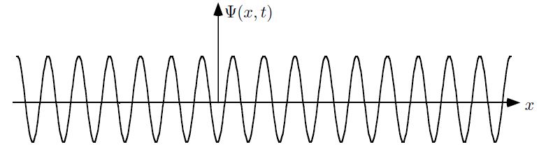
We also know that the wavelength we are talking about it here is not the wavelength of some electromagnetic wave, like light. It’s the wavelength of a de Broglie wave, i.e. a matter wave: such wave is represented by an (oscillating) complex number – so we need to keep track of a real and an imaginary part – representing a so-called probability amplitude Ψ(x, t) whose modulus squared (│Ψ(x, t)│²) is the probability of actually detecting the electron at point x at time t. [The purists will say that complex numbers can’t oscillate – but I am sure you get the idea.]

You should read the phrase above twice: we cannot know where the electron actually is. We can only calculate probabilities (and, of course, compare them with the probabilities we get from experiments). Hence, when the wave function tells us the probability is greatest at point x at time t, then we may be lucky when we actually probe point x at time t and find it there, but it may also not be there. In fact, the probability of finding it exactly at some point x at some definite time t is zero. That’s just a characteristic of such probability density functions: we need to probe some region Δx in some time interval Δt.

If you think that is not very satisfactory, there’s actually a very common-sense explanation that has nothing to do with quantum mechanics: our scientific instruments do not allow us to go beyond a certain scale anyway. Indeed, the resolution of the best electron microscopes, for example, is some 50 picometer (1 pm = 1×10^–12 m): that’s small (and resolutions get higher by the year), but so it implies that we are not looking at points – as defined in math that is: so that’s something with zero dimension – but at pixels of size Δx = 50×10^–12 m.

The same goes for time. Time is measured by atomic clocks nowadays but even these clocks do ‘tick’, and these ‘ticks’ are discrete. Atomic clocks take advantage of the property of atoms to resonate at extremely consistent frequencies. I’ll say something more about resonance soon – because it’s very relevant for what I am writing about in this post – but, for the moment, just note that, for example, Caesium-133 (which was used to build the first atomic clock) oscillates at 9,192,631,770 cycles per second. In fact, the International Bureau of Standards and Weights re-defined the (time) second in 1967 to correspond to “the duration of 9,192,631,770 periods of the radiation corresponding to the transition between the two hyperfine levels of the ground state of the Caesium-133 atom at rest at a temperature of 0 K.”

Don’t worry about it: the point to note is that when it comes to measuring time, we also have an uncertainty. Now, when using this Caesium-133 atomic clock, this uncertainty would be in the range of ±9.2×10^–9 seconds (so that’s nanoseconds: 1 ns = 1×10^–9 s), because that’s the rate at which this clock ‘ticks’. However, there are other (much more plausible) ways of measuring time: some of the unstable baryons have lifetimes in the range of a few picoseconds only (1 ps = 1×10^–12 s) and the really unstable ones – known as baryon resonances – have lifetimes in the 1×10^–22 to 1×10^–24 s range. This we can only measure because they leave some trace after these particle collisions in particle accelerators and, because we have some idea about their speed, we can calculate their lifetime from the (limited) distance they travel before disintegrating. The thing to remember is that for time also, we have to make do with time pixels instead of time points, so there is a Δt as well. [In case you wonder what baryons are: they are particles consisting of three quarks, and the proton and the neutron are the most prominent (and most stable) representatives of this family of particles.]

So what’s the size of an electron? Well… It depends. We need to distinguish two very different things: (1) the size of the area where we are likely to find the electron, and (2) the size of the electron itself. Let’s start with the latter, because that’s the easiest question to answer: there is a so-called classical electron radius r_e, which is also known as the Thompson scattering length, which has been calculated as:

$r_\mathrm{e} = \frac{1}{4\pi\varepsilon_0}\frac{e^2}{m_{\mathrm{e}} c^2} = 2.817 940 3267(27) \times 10^{-15} \mathrm{m}$ As for the constants in this formula, you know these by now: the speed of light c, the electron charge e, its mass m_e, and the permittivity of free space ε_e. For whatever it’s worth (because you should note that, in quantum mechanics, electrons do not have a size: they are treated as point-like particles, so they have a point charge and zero dimension), that’s small. It’s in the femtometer range (1 fm = 1×10^–15 m). You may or may not remember that the size of a proton is in the femtometer range as well – 1.7 fm to be precise – and we had a femtometer size estimate for quarks as well: 0.7 m. So we have the rather remarkable result that the much heavier proton (its rest mass is 938 MeV/c²sas opposed to only 0.511 MeV MeV/c², so the proton is 1835 times heavier) is 1.65 times smaller than the electron. That’s something to be explored later: for the moment, we’ll just assume the electron wiggles around a bit more – exactly because it’s lighter. Here you just have to note that this ‘classical’ electron radius does measure something: it’s something ‘hard’ and ‘real’ because it scatters, absorbs or deflects photons (and/or other particles). In one of my previous posts, I explained how particle accelerators probe things at the femtometer scale, so I’ll refer you to that post (End of the Road to Reality?) and move on to the next question.

The question concerning the area where we are likely to detect the electron is more interesting in light of the topic of this post (the nature of these matter waves). It is given by that wave function and, from my previous post, you’ll remember that we’re talking the nanometer scale here (1 nm = 1×10^–9 m), so that’s a million times larger than the femtometer scale. Indeed, we’ve calculated a de Broglie wavelength of 0.33 nanometer for relatively slow-moving electrons (electrons in orbit), and the slits used in single- or double-slit experiments with electrons are also nanotechnology. In fact, now that we are here, it’s probably good to look at those experiments in detail.

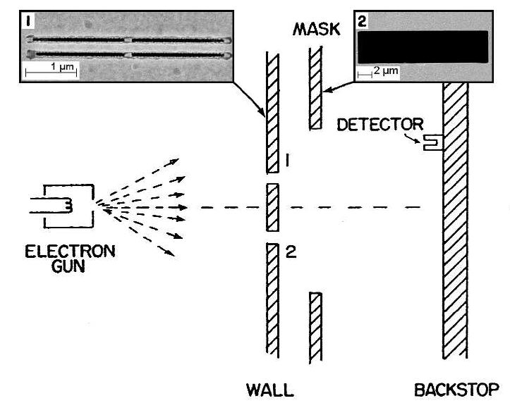
The illustration below relates the actual experimental set-up of a double-slit experiment performed in 2012 to Feynman’s 1965 thought experiment. Indeed, in 1965, the nanotechnology you need for this kind of experiment was not yet available, although the phenomenon of electron diffraction had been confirmed experimentally already in 1925 in the famous Davisson-Germer experiment. [It’s famous not only because electron diffraction was a weird thing to contemplate at the time but also because it confirmed the de Broglie hypothesis only two years after Louis de Broglie had advanced it!]. But so here is the experiment which Feynman thought would never be possible because of technology constraints:

The insert in the upper-left corner shows the two slits: they are each 50 nanometer wide (50×10^–9 m) and 4 micrometer tall (4×10^–6 m). [The thing in the middle of the slits is just a little support. Please do take a few seconds to contemplate the technology behind this feat: 50 nm is 50 millionths of a millimeter. Try to imagine dividing one millimeter in ten, and then one of these tenths in ten again, and again, and once again, again, and again. You just can’t imagine that, because our mind is used to addition/subtraction and – to some extent – with multiplication/division: our mind can’t deal with with exponentiation really – because it’s not a everyday phenomenon.] The second inset (in the upper-right corner) shows the mask that can be moved to close one or both slits partially or completely.

Now, 50 nanometer is 150 times larger than the 0.33 nanometer range we got for ‘our’ electron, but it’s small enough to show diffraction and/or interference. [In fact, in this experiment (done by Bach, Pope, Liou and Batelaan from the University of Nebraska-Lincoln less than two years ago indeed), the beam consisted of electrons with an (average) energy of 600 eV and a de Broglie wavelength of 50 picometer. So that’s like the electrons used in electron microscopes. 50 pm is 6.6 times smaller than the 0.33 nm wavelength we calculated for our low-energy (70 eV) electron – but then the energy and the fact these electrons are guided in electromagnetic fields explain the difference. Let’s go to the results.

The illustration below shows the predicted pattern next to the observed pattern for the two scenarios:

We first close slit 2, let a lot of electrons go through it, and so we get a pattern described by the probability density function P₁ = │Φ₁│². Here we see no interference but a typical diffraction pattern: the intensity follows a more or less normal (i.e. Gaussian) distribution. We then close slit 1 (and open slit 2 again), again let a lot of electrons through, and get a pattern described by the probability density function P₂ = │Φ₂│². So that’s how we get P₁ and P₂.
We then open both slits, let a whole electrons through, and get according to the pattern described by probability density function P₁₂ = │Φ₁+Φ₂│², which we get not from adding the probabilities P₁ and P₂(hence, P₁₂ ≠ P₁ + P₂) – as one would expect if electrons would behave like particles – but from adding the probability amplitudes. We have interference, rather than diffraction.

But so what exactly is interfering? Well… The electrons. But that can’t be, can it?

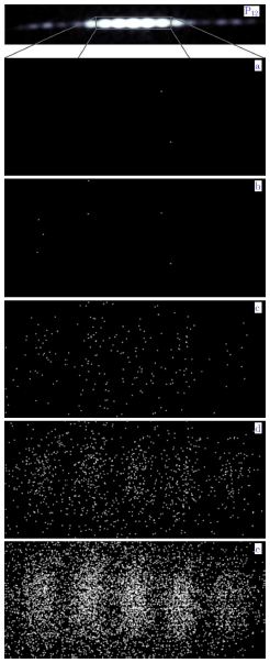
The electrons are obviously particles, as evidenced from the impact they make – one by one – as they hit the screen as shown below. [If you want to know what screen, let me quote the researchers: “The resulting patterns were magnified by an electrostatic quadrupole lens and imaged on a two-dimensional microchannel plate and phosphorus screen, then recorded with a charge-coupled device camera. […] To study the build-up of the diffraction pattern, each electron was localized using a “blob” detection scheme: each detection was replaced by a blob, whose size represents the error in the localization of the detection scheme. The blobs were compiled together to form the electron diffraction patterns.” So there you go.]

Look carefully at how this interference pattern becomes ‘reality’ as the electrons hit the screen one by one. And then say it: WAW !

Indeed, as predicted by Feynman (and any other physics professor at the time), even if the electrons go through the slits one by one, they will interfere – with themselves so to speak. [In case you wonder if these electrons really went through one by one, let me quote the researchers once again: “The electron source’s intensity was reduced so that the electron detection rate in the pattern was about 1 Hz. At this rate and kinetic energy, the average distance between consecutive electrons was 2.3 × 106 meters. This ensures that only one electron is present in the 1 meter long system at any one time, thus eliminating electron-electron interactions.” You don’t need to be a scientist or engineer to understand that, isn’t it?]

While this is very spooky, I have not seen any better way to describe the reality of the de Broglie wave: the particle is not some point-like thing but a matter wave, as evidenced from the fact that it does interfere with itself when forced to move through two slits – or through one slit, as evidenced by the diffraction patterns built up in this experiment when closing one of the two slits: the electrons went through one by one as well!

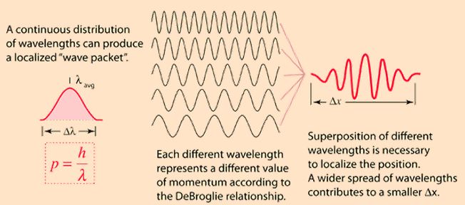
But so how does it relate to the characteristics of that wave packet which I described in my previous post? Let me sum up the salient conclusions from that discussion:

The wavelength λ of a wave packet is calculated directly from the momentum by using de Broglie‘s second relation: λ = h/p. In this case, the wavelength of the electrons averaged 50 picometer. That’s relatively small as compared to the width of the slit (50 nm) – a thousand times smaller actually! – but, as evidenced by the experiment, it’s small enough to show the ‘reality’ of the de Broglie wave.
From a math point (but, of course, Nature does not care about our math), we can decompose the wave packet in a finite or infinite number of component waves. Such decomposition is referred to, in the first case (finite number of composite waves or discrete calculus) as a Fourier analysis, or, in the second case, as a Fourier transform. A Fourier transform maps our (continuous) wave function, Ψ(x), to a (continuous) wave function in the momentum space, which we noted as φ(p). [In fact, we noted it as Φ(p) but I don’t want to create confusion with the Φ symbol used in the experiment, which is actually the wave function in space, so Ψ(x) is Φ(x) in the experiment – if you know what I mean.] The point to note is that uncertainty about momentum is related to uncertainty about position. In this case, we’ll have pretty standard electrons (so not much variation in momentum), and so the location of the wave packet in space should be fairly precise as well.
The group velocity of the wave packet (v_g) – i.e. the envelope in which our Ψ wave oscillates – equals the speed of our electron (v), but the phase velocity (i.e. the speed of our Ψ wave itself) is superluminal: we showed it’s equal to (v_p) = E/p = c²/v = c/β, with β = v/c, so that’s the ratio of the speed of our electron and the speed of light. Hence, the phase velocity will always be superluminal but will approach c as the speed of our particle approaches c. For slow-moving particles, we get astonishing values for the phase velocity, like more than a hundred times the speed of light for the electron we looked at in our previous post. That’s weird but it does not contradict relativity: if it helps, one can think of the wave packet as a modulation of an incredibly fast-moving ‘carrier wave’.

Is any of this relevant? Does it help you to imagine what the electron actually is? Or what that matter wave actually is? Probably not. You will still wonder: How does it look like? What is it in reality?

That’s hard to say. If the experiment above does not convey any ‘reality’ according to you, then perhaps the illustration below will help. It’s one I have used in another post too (An Easy Piece: Introducing Quantum Mechanics and the Wave Function). I took it from Wikipedia, and it represents “the (likely) space in which a single electron on the 5d atomic orbital of an atom would be found.” The solid body shows the places where the electron’s probability density (so that’s the squared modulus of the probability amplitude) is above a certain value – so it’s basically the area where the likelihood of finding the electron is higher than elsewhere. The hue on the colored surface shows the complex phase of the wave function.

So… Does this help?

You will wonder why the shape is so complicated (but it’s beautiful, isn’t it?) but that has to do with quantum-mechanical calculations involving quantum-mechanical quantities such as spin and other machinery which I don’t master (yet). I think there’s always a bit of a gap between ‘first principles’ in physics and the ‘model’ of a real-life situation (like a real-life electron in this case), but it’s surely the case in quantum mechanics! That being said, when looking at the illustration above, you should be aware of the fact that you are actually looking at a 3D representation of the wave function of an electron in orbit.

Indeed, wave functions of electrons in orbit are somewhat less random than – let’s say – the wave function of one of those baryon resonances I mentioned above. As mentioned in my Not So Easy Piece, in which I introduced the Schrödinger equation (i.e. one of my previous posts), they are solutions of a second-order partial differential equation – known as the Schrödinger wave equation indeed – which basically incorporates one key condition: these solutions – which are (atomic or molecular) ‘orbitals’ indeed – have to correspond to so-called stationary states or standing waves. Now what’s the ‘reality’ of that?

The illustration below comes from Wikipedia once again (Wikipedia is an incredible resource for autodidacts like me indeed) and so you can check the article (on stationary states) for more details if needed. Let me just summarize the basics:

A stationary state is called stationary because the system remains in the same ‘state’ independent of time. That does not mean the wave function is stationary. On the contrary, the wave function changes as function of both time and space – Ψ = Ψ(x, t) remember? – but it represents a so-called standing wave.
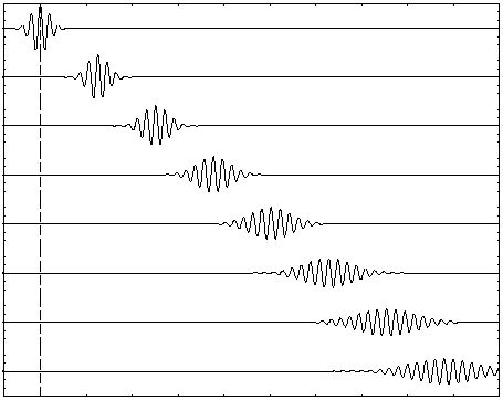
Each of these possible states corresponds to an energy state, which is given through the de Broglie relation: E = hf. So the energy of the state is proportional to the oscillation frequency of the (standing) wave, and Planck’s constant is the factor of proportionality. From a formal point of view, that’s actually the one and only condition we impose on the ‘system’, and so it immediately yields the so-called time-independent Schrödinger equation, which I briefly explained in the above-mentioned Not So Easy Piece (but I will not write it down here because it would only confuse you even more). Just look at these so-called harmonic oscillators below:

A and B represent a harmonic oscillator in classical mechanics: a ball with some mass m (mass is a measure for inertia, remember?) on a spring oscillating back and forth. In case you’d wonder what the difference is between the two: both the amplitude as well as the frequency of the movement are different. 🙂 A spring and a ball?

It represents a simple system. A harmonic oscillation is basically a resonance phenomenon: springs, electric circuits,… anything that swings, moves or oscillates (including large-scale things such as bridges and what have you – in his 1965 Lectures (Vol. I-23), Feynman even discusses resonance phenomena in the atmosphere in his Lectures) has some natural frequency ω₀, also referred to as the resonance frequency, at which it oscillates naturally indeed: that means it requires (relatively) little energy to keep it going. How much energy it takes exactly to keep them going depends on the frictional forces involved: because the springs in A and B keep going, there’s obviously no friction involved at all. [In physics, we say there is no damping.] However, both springs do have a different k (that’s the key characteristic of a spring in Hooke’s Law, which describes how springs work), and the mass m of the ball might be different as well. Now, one can show that the period of this ‘natural’ movement will be equal to t₀ = 2π/ω₀= 2π(m/k)^1/2or that ω₀= (m/k)^–1/2. So we’ve got a A and a B situation which differ in k and m. Let’s go to the so-called quantum oscillator, illustrations C to H.

C to H in the illustration are six possible solutions to the Schrödinger Equation for this situation. The horizontal axis is position (and so time is the variable) – but we could switch the two independent variables easily: as I said a number of times already, time and space are interchangeable in the argument representing the phase (θ) of a wave provided we use the right units (e.g. light-seconds for distance and seconds for time): θ = ωt – kx. Apart from the nice animation, the other great thing about these illustrations – and the main difference with resonance frequencies in the classical world – is that they show both the real part (blue) as well as the imaginary part (red) of the wave function as a function of space (fixed in the x axis) and time (the animation).

Is this ‘real’ enough? If it isn’t, I know of no way to make it any more ‘real’. Indeed, that’s key to understanding the nature of matter waves: we have to come to terms with the idea that these strange fluctuating mathematical quantities actually represent something. What? Well… The spooky thing that leads to the above-mentioned experimental results: electron diffraction and interference.

Let’s explore this quantum oscillator some more. Another key difference between natural frequencies in atomic physics (so the atomic scale) and resonance phenomena in ‘the big world’ is that there is more than one possibility: each of the six possible states above corresponds to a solution and an energy state indeed, which is given through the de Broglie relation: E = hf. However, in order to be fully complete, I have to mention that, while G and H are also solutions to the wave equation, they are actually not stationary states. The illustration below – which I took from the same Wikipedia article on stationary states – shows why. For stationary states, all observable properties of the state (such as the probability that the particle is at location x) are constant. For non-stationary states, the probabilities themselves fluctuate as a function of time (and space of obviously), so the observable properties of the system are not constant. These solutions are solutions to the time-dependent Schrödinger equation and, hence, they are, obviously, time-dependent solutions.

We can find these time-dependent solutions by superimposing two stationary states, so we have a new wave function Ψ_N which is the sum of two others: Ψ_N = Ψ₁ + Ψ₂. [If you include the normalization factor (as you should to make sure all probabilities add up to 1), it’s actually Ψ_N = (2^–1/2)(Ψ₁ + Ψ₂).] So G and H above still represent a state of a quantum harmonic oscillator (with a specific energy level proportional to h), but so they are not standing waves.

Let’s go back to our electron traveling in a more or less straight path. What’s the shape of the solution for that one? It could be anything. Well… Almost anything. As said, the only condition we can impose is that the envelope of the wave packet – its ‘general’ shape so to say – should not change. That because we should not have dispersion – as illustrated below. [Note that this illustration only represent the real or the imaginary part – not both – but you get the idea.]

That being said, if we exclude dispersion (because a real-life electron traveling in a straight line doesn’t just disappear – as do dispersive wave packets), then, inside of that envelope, the weirdest things are possible – in theory that is. Indeed, Nature does not care much about our Fourier transforms. So the example below, which shows a theoretical wave packet (again, the real or imaginary part only) based on some theoretical distribution of the wave numbers of the (infinite number) of component waves that make up the wave packet, may or may not represent our real-life electron. However, if our electron has any resemblance to real-life, then I would expect it to not be as well-behaved as the theoretical one that’s shown below.

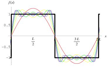
The shape above is usually referred to as a Gaussian wave packet, because of the nice normal (Gaussian) probability density functions that are associated with it. But we can also imagine a ‘square’ wave packet: a somewhat weird shape but – in terms of the math involved – as consistent as the smooth Gaussian wave packet, in the sense that we can demonstrate that the wave packet is made up of an infinite number of waves with an angular frequency ω that is linearly related to their wave number k, so the dispersion relation is ω = ak + b. [Remember we need to impose that condition to ensure that our wave packet will not dissipate (or disperse or disappear – whatever term you prefer.] That’s shown below: a Fourier analysis of a square wave.

While we can construct many theoretical shapes of wave packets that respect the ‘no dispersion!’ condition, we cannot know which one will actually represent that electron we’re trying to visualize. Worse, if push comes to shove, we don’t know if these matter waves (so these wave packets) actually consist of component waves (or time-independent stationary states or whatever).

[…] OK. Let me finally admit it: while I am trying to explain you the ‘reality’ of these matter waves, we actually don’t know how real these matter waves actually are. We cannot ‘see’ or ‘touch’ them indeed. All that we know is that (i) assuming their existence, and (ii) assuming these matter waves are more or less well-behaved (e.g. that actual particles will be represented by a composite wave characterized by a linear dispersion relation between the angular frequencies and the wave numbers of its (theoretical) component waves) allows us to do all that arithmetic with these (complex-valued) probability amplitudes. More importantly, all that arithmetic with these complex numbers actually yields (real-valued) probabilities that are consistent with the probabilities we obtain through repeated experiments. So that’s what’s real and ‘not so real’ I’d say.

Indeed, the bottom-line is that we do not know what goes on inside that envelope. Worse, according to the commonly accepted Copenhagen interpretation of the Uncertainty Principle (and tons of experiments have been done to try to overthrow that interpretation – all to no avail), we never will.

Some content on this page was disabled on June 20, 2020 as a result of a DMCA takedown notice from Michael A. Gottlieb, Rudolf Pfeiffer, and The California Institute of Technology. You can learn more about the DMCA here:

https://wordpress.com/support/copyright-and-the-dmca/
Some content on this page was disabled on June 20, 2020 as a result of a DMCA takedown notice from Michael A. Gottlieb, Rudolf Pfeiffer, and The California Institute of Technology. You can learn more about the DMCA here:

https://wordpress.com/support/copyright-and-the-dmca/

Re-visiting the matter wave (I)

Pre-scriptum (dated 26 June 2020): This post did not suffer from the DMCA take-down of some material. It is, therefore, still quite readable—even if my views on these matters have evolved quite a bit as part of my realist interpretation of QM. However, I now think de Broglie’s intuition in regard to particles being waves was correct but that he should have used a circular rather than a linear wave concept. Also, the idea of a particle being some wave packet is erroneous. It leads to the kind of contradictions I already start mentioning here, such as super-luminous velocities and other nonsense. Such critique is summarized in my paper on de Broglie’s wave concept. I also discuss it in the context of analyzing wavefunction math in the context of signal transmission in a crystal lattice.

Original post:

In my previous posts, I introduced a lot of wave formulas. They are essential to understanding waves – both real ones (e.g. electromagnetic waves) as well as probability amplitude functions. Probability amplitude function is quite a mouthful so let me call it a matter wave, or a de Broglie wave. The formulas are necessary to create true understanding – whatever that means to you – because otherwise we just keep on repeating very simplistic but nonsensical things such as ‘matter behaves (sometimes) like light’, ‘light behaves (sometimes) like matter’ or, combining both, ‘light and matter behave like wavicles’. Indeed: what does ‘like‘ mean? Like the same but different? 🙂 So that means it’s different. Let’s therefore re-visit the matter wave (i.e. the de Broglie wave) and point out the differences with light waves.

In fact, this post actually has its origin in a mistake in a post scriptum of a previous post (An Easy Piece: On Quantum Mechanics and the Wave Function), in which I wondered what formula to use for the energy E in the (first) de Broglie relation E = hf (with f the frequency of the matter wave and h the Planck constant). Should we use (a) the kinetic energy of the particle, (b) the rest mass (mass is energy, remember?), or (c) its total energy? So let us first re-visit these de Broglie relations which, you’ll remember, relate energy and momentum to frequency (f) and wavelength (λ) respectively with the Planck constant as the factor of proportionality:

E = hf and p = h/λ

The de Broglie wave

I first tried kinetic energy in that E = hf equation. However, if you use the kinetic energy formula (K.E. = mv²/2, with v the velocity of the particle), then the second de Broglie relation (p = h/λ) does not come out right. The second de Broglie relation has the wavelength λ on the right side, not the frequency f. But it’s easy to go from one to the other: frequency and wavelength are related through the velocity of the wave (v). Indeed, the number of cycles per second (i.e. the frequency f) times the length of one cycle (i.e. the wavelength λ) gives the distance traveled by the wave per second, i.e. its velocity v. So fλ = v. Hence, using that kinetic energy formula and that very obvious fλ = v relation, we can write E = hf as mv²/2 = v/λ and, hence, after moving one of the two v’s in v² (and the 1/2 factor) on the left side to the right side of this equation, we get mv = 2h/λ. So there we are:

p = mv = 2h/λ.

Well… No. The second de Broglie relation is just p = h/λ. There is no factor 2 in it. So what’s wrong?

A factor of 2 in an equation like this surely doesn’t matter, does it? It does. We are talking tiny wavelengths here but a wavelength of 1 nanometer (1×10^–9 m) – this is just an example of the scale we’re talking about here – is not the same as a wavelength of 0.5 nm. There’s another problem too. Let’s go back to our an example of an electron with a mass of 9.1×10^–31kg (that’s very tiny, and so you’ll usually see it expressed in a unit that’s more appropriate to the atomic scale), moving about with a velocity of 2.2×10⁶m/s (that’s the estimated speed of orbit of an electron around a hydrogen nucleus: it’s fast (2,200 km per second), but still less than 1% of the speed of light), and let’s do the math.

[Before I do the math, however, let me quickly insert a line on that ‘other unit’ to measure mass. You will usually see it written down as eV, so that’s electronvolt. Electronvolt is a measure of energy but that’s OK because mass is energy according to Einstein’s mass-energy equation: E = mc². The point to note is that the actual measure for mass at the atomic scale is eV/c², so we make the unit even smaller by dividing the eV (which already is a very tiny amount of energy) by c²: 1 eV/c²corresponds to 1.782662×10⁻³⁶ kg, so the mass of our electron (9.1×10^–31kg) is about 510,000 eV/c², or 0.510 MeV/c². I am spelling it out because you will often just see 0.510 MeV in older or more popular publications, but so don’t forget that c²factor. As for the calculations below, I just stick to the kg and m measures because they make the dimensions come out right.]

According to our kinetic energy formula (K.E. = mv²/2), these mass and velocity values correspond to an energy value of 22 ×10⁻¹⁹ Joule (the Joule is the so-called SI unit for energy – don’t worry about it right now). So, from the first de Broglie equation (f = E/h) – and using the right value for Planck’s constant (6.626 J·s), we get a frequency of 3.32×10¹⁵ hertz (hertz just means oscillations per second as you know). Now, using v once again, and fλ = v, we see that corresponds to a wavelength of 0.66 nanometer (0.66×10⁻⁹ m). [Just take the numbers and do the math.]

However, if we use the second de Broglie relation, which relates wavelength to momentum instead of energy, then we get 0.33 nanometer (0.33×10⁻⁹ m), so that’s half of the value we got from the first equation. So what is it: 0.33 or 0.66 nm? It’s that factor 2 again. Something is wrong.

It must be that kinetic energy formula. You’ll say we should include potential energy or something. No. That’s not the issue. First, we’re talking a free particle here: an electron moving in space (a vacuum) with no external forces acting on it, so it’s a field-free space (or a region of constant potential). Second, we could, of course, extend the analysis and include potential energy, and show how it’s converted to kinetic energy (like a stone falling from 100 m to 50 m: potential energy gets converted into kinetic energy) but making our analysis more complicated by including potential energy as well will not solve our problem here: it will only make you even more confused.

Then it must be some relativistic effect you’ll say. No. It’s true the formula for kinetic energy above only holds for relatively low speeds (as compared to light, so ‘relatively’ low can be thousands of km per second) but that’s not the problem here: we are talking electrons moving at non-relativistic speeds indeed, so their mass or energy is not (or hardly) affected by relativistic effects and, hence, we can indeed use the more simple non-relativistic formulas.

The real problem we’re encountering here is not with the equations: it’s the simplistic model of our wave. We are imagining one wave here indeed, with a single frequency, a single wavelength and, hence, one single velocity – which happens to coincide with the velocity of our particle. Such wave cannot possibly represent an actual de Broglie wave: the wave is everywhere and, hence, the particle it represents is nowhere. Indeed, a wave defined by a specific wavelength λ (or a wave number k = 2π/λ if we’re using complex number notation) and a specific frequency f or period T (or angular frequency ω = 2π/T = 2πf) will have a very regular shape – such as Ψ= Aeⁱ⁽^ωt-kx) and, hence, the probability of actually locating that particle at some specific point in space will be the same everywhere: |Ψ|²= |Aeⁱ⁽^ωt-kx)|²= A². [If you are confused about the math here, I am sorry but I cannot re-explain this once again: just remember that our de Broglie wave represents probability amplitudes – so that’s some complex number Ψ = Ψ(x, t) depending on space and time – and that we need to take the modulus squared of that complex number to get the probability associated with some (real) value x (i.e. the space variable) and some value t (i.e. the time variable).]

So the actual matter wave of a real-life electron will be represented by a wave train, or a wave packet as it is usually referred to. Now, a wave packet is described by (at least) two types of wave velocity:

The so-called group velocity: the group velocity of a wave is denoted by v_gand is the velocity of the wave packet as a whole is traveling. Wikipedia defines it as “the velocity with which the overall shape of the waves’ amplitudes — known as the modulation or envelope of the wave — propagates through space.”
The so-called phase velocity: the phase velocity is denoted by v_p and is what we usually associate with the velocity of a wave. It is just what it says it is: the rate at which the phase of the (composite) wave travels through space.

The term between brackets above – ‘composite’ – already indicates what it’s all about: a wave packet is to be analyzed as a composite wave: so it’s a wave composed of a finite or infinite number of component waves which all have their own wave number k and their own angular frequency ω. So the mistake we made above is that, naively, we just assumed that (i) there is only one simple wave (and, of course, there is only one wave, but it’s not a simple one: it’s a composite wave), and (ii) that the velocity v of our electron would be equal to the velocity of that wave. Now that we are a little bit more enlightened, we need to answer two questions in regard to point (ii):

Why would that be the case?
If it’s is the case, then what wave velocity are we talking about: the group velocity or the phase velocity?

To answer both questions, we need to look at wave packets once again, so let’s do that. Just to visualize things, I’ll insert – once more – that illustration you’ve seen in my other posts already:

The de Broglie wave packet

The Wikipedia article on the group velocity of a wave has wonderful animations, which I would advise you to look at in order to make sure you are following me here. There are several possibilities:

The phase velocity and the group velocity are the same: that’s a rather unexciting possibility but it’s the easiest thing to work with and, hence, most examples will assume that this is the case.
The group and phase velocity are not the same, but our wave packet is ‘stable’, so to say. In other words, the individual peaks and troughs of the wave within the envelope travel at a different speed (the phase velocity v_g), but the envelope as a whole (so the wave packet as such) does not get distorted as it travels through space.
The wave packet dissipates: in this case, we have a constant group velocity, but the wave packet delocalizes. Its width increases over time and so the wave packet diffuses – as time goes by – over a wider and wider region of space, until it’s actually no longer there. [In case you wonder why it did not group this third possibility under (2): it’s a bit difficult to assign a fixed phase velocity to a wave like this.]

How the wave packet will behave depends on the characteristics of the component waves. To be precise, it will depend on their angular frequency and their wave number and, hence, their individual velocities. First, note the relationship between these three variables: ω = 2πf and k = 2π/λ so ω/k = fλ = v. So these variables are not independent: if you have two values (e.g. v and k), you also have the third one (ω). Secondly, note that the component waves of our wave packet will have different wavelengths and, hence, different wave numbers k.

Now, the de Broglie relation p = ħk (i.e. the same relation as p = h/λ but we replace λ with 2π/k and then ħ is the so-called reduced Planck constant ħ = h/2π) makes it obvious that different wave numbers k correspond to different values p for the momentum of our electron, so allowing for a spread in k (or a spread in λ as illustrates above) amounts to allowing for some spread in p. That’s where the uncertainty principle comes in – which I actually derived from a theoretical wave function in my post on Fourier transforms and conjugate variables. But so that’s not something I want to dwell on here.

We’re interested in the ω’s. What about them? Well… ω can take any value really – from a theoretical point of view that is. Now you’ll surely object to that from a practical point of view, because you know what it implies: different velocities of the component waves. But you can’t object in a theoretical analysis like this. The only thing we could possible impose as a constraint is that our wave packet should not dissipate – so we don’t want it to delocalize and/or vanish after a while because we’re talking about some real-life electron here, and so that’s a particle which just doesn’t vanish like that.

To impose that condition, we need to look at the so-called dispersion relation. We know that we’ll have a whole range of wave numbers k, but so what values should ω take for a wave function to be ‘well-behaved’, i.e. not disperse in our case? Let’s first accept that k is some variable, the independent variable actually, and so then we associate some ω with each of these values k. So ω becomes the dependent variable (dependent on k that is) and that amounts to saying that we have some function ω = ω(k).

What kind of function? Well… It’s called the dispersion relation – for rather obvious reasons: because this function determines how the wave packet will behave: non-dispersive or – what we don’t want here – dispersive. Indeed, there are several possibilities:

The speed of all component waves is the same: that means that the ratio ω/k = v is the same for all component waves. Now that’s the case only if ω is directly proportional to k, with the factor of proportionality equal to v. That means that we have a very simple dispersion relation: ω = αk with α some constant equal to the velocity of the component waves as well as the group and phase velocity of the composite wave. So all velocities are just the same (v = v_p = v_g = α) and we’re in the first of the three cases explained at the beginning of this section.
There is a linear relation between ω and k but no direct proportionality, so we write ω = αk + β, in which β can be anything but not some function of k. So we allow different wave speeds for the component waves. The phase velocity will, once again, be equal to the ratio of the angular frequency and the wave number of the composite wave (whatever that is), but what about the group velocity, i.e. the velocity of our electron in this example? Well… One can show – but I will not do it here because it is quite a bit of work – that the group velocity of the wave packet will be equal to v_g = dω/dk, i.e. the (first-order) derivative of ω with respect to k. So, if we want that wave packet to travel at the same speed of our electron (which is what we want of course because, otherwise, the wave packet would obviously not represent our electron), we’ll have to impose that dω/dk (or ∂ω/∂k if you would want to introduce more independent variables) equals v. In short, we have the condition that dω/dk = d(αk + β)/dk = α = k.
If the relation between ω and k is non-linear, well… Then we have none of the above. Hence, we then have a wave packet that gets distorted and stretched out and actually vanishes after a while. That case surely does not represent an electron.

Back to the de Broglie wave relations

Indeed, it’s now time to go back to our de Broglie relations – E = hf and p = h/λ and the question that sparked the presentation above: what formula to use for E? Indeed, for p it’s easy: we use p = mv and, if you want to include the case of relativistic speeds, you will write that formula in a more sophisticated way by making it explicit that the mass m is the relativistic mass m = γm₀: the rest mass multiplied with a factor referred to as the Lorentz factor which, I am sure, you have seen before: γ = (1 – v²/c²)^–1/2. At relativistic speeds (i.e. speeds close to c), this factor makes a difference: it adds mass to the rest mass. So the mass of a particle can be written as m = γm₀, with m₀ denoting the rest mass. At low speeds (e.g. 1% of the speed of light – as in the case of our electron), m will hardly differ from m₀ and then we don’t need this Lorentz factor. It only comes into play at higher speeds.

At this point, I just can’t resist a small digression. It’s just to show that it’s not ‘relativistic effects’ that cause us trouble in finding the right energy equation for our E = hf relation. What’s kinetic energy? Well… There’s a few definitions – such as the energy gathered through converting potential energy – but one very useful definition in the current context is the following: kinetic energy is the excess of a particle over its rest mass energy. So when we’re looking at high-speed or high-energy particles, we will write the kinetic energy as K.E. = mc²– m₀c²= (m – m₀)c²= γm₀c²– m₀c²= m₀c²(γ – 1).Before you think I am trying to cheat you: where is the v of our particle? [To make it specific: think about our electron once again but not moving at leisure this time around: imagine it’s speeding at a velocity very close to c in some particle accelerator. Now, v is close to c but not equal to c and so it should not disappear. […]

It’s in the Lorentz factor γ = (1 – v²/c²)^–1/2.

Now, we can expand γ into a binomial series (it’s basically an application of the Taylor series – but just check it online if you’re in doubt), so we can write γ as an infinite sum of the following terms: γ = 1 + (1/2)·v²/c²+ (3/8)·v⁴/c⁴+ (3/8)·v⁴/c⁴+ (5/16)·v⁶/c⁶+ … etcetera. [The binomial series is an infinite Taylor series, so it’s not to be confused with the (finite) binomial expansion.] Now, when we plug this back into our (relativistic) kinetic energy equation, we can scrap a few things (just do it) to get where I want to get:

K.E. = (1/2)·m₀v²+ (3/8)·m₀v⁴/c²+ (5/16)·m₀v⁶/c⁴+ … etcetera

So what? Well… That’s it – for the digression at least: see how our non-relativistic formula for kinetic energy (K.E. = m₀v²/2 is only the first term of this series and, hence, just an approximation: at low speeds, the second, third etcetera terms represent close to nothing (and more close to nothing as you check out the fourth, fifth etcetera terms). OK, OK… You’re getting tired of these games. So what? Should we use this relativistic kinetic energy formula in the de Broglie relation?

No. As mentioned above already, we don’t need any relativistic correction, but the relativistic formula above does come in handy to understand the next bit. What’s the next bit about?

Well… It turns out that we actually do have to use the total energy – including (the energy equivalent to) the rest mass of our electron – in the de Broglie relation E = hf.

WHAT!?

If you think a few seconds about the math of this – so we’d use γm₀c²instead of (1/2)m₀v²(so we use the speed of light instead of the speed of our particle) – you’ll realize we’ll be getting some astronomical frequency (we got that already but so here we are talking some kind of truly fantastic frequency) and, hence, combining that with the wavelength we’d derive from the other de Broglie equation (p = h/λ) we’d surely get some kind of totally unreal speed. Whatever it is, it will surely have nothing to do with our electron, does it?

Let’s go through the math.

The wavelength is just the same as that one given by p = h/λ, so we have λ = 0.33 nanometer. Don’t worry about this. That’s what it is indeed. Check it out online: it’s about a thousand times smaller than the wavelength of (visible) light but that’s OK. We’re talking something real here. That’s why electron microscopes can ‘see’ stuff that light microscopes can’t: their resolution is about a thousand times higher indeed.

But so when we take the first equation once again (E =hf) and calculate the frequency from f = γm₀c²/h, we get an frequency f in the neighborhood of 12.34×10¹⁹herz. So that gives a velocity of v = fλ = 4.1×10¹⁰meter per second (m/s). But… THAT’S MORE THAN A HUNDRED TIMES THE SPEED OF LIGHT. Surely, we must have got it wrong.

We don’t. The velocity we are calculating here is the phase velocity v_p of our matter wave – and IT’S REAL! More in general, it’s easy to show that this phase velocity is equal to v_p = fλ = E/p = (γm₀c²/h)·(h/γm₀v) = c²/v. Just fill in the values for c and v (3×10⁸ and 2.2×10⁶ respectively and you will get the same answer.

But that’s not consistent with relativity, is it? It is: phase velocities can be (and, in fact, usually are – as evidenced by our real-life example) superluminal as they say – i.e. much higher than the speed of light. However, because they carry no information – the wave packet shape is the ‘information’, i.e. the (approximate) location of our electron – such phase velocities do not conflict with relativity theory. It’s like amplitude modulation, like AM radiowaves): the modulation of the amplitude carries the signal, not the carrier wave.

The group velocity, on the other hand, can obviously not be faster than c and, in fact, should be equal to the speed of our particle (i.e. the electron). So how do we calculate that? We don’t have any formula ω(k) here, do we? No. But we don’t need one. Indeed, we can write:

v_g= ∂ω/∂k = ∂(E/ ħ)/∂(p/ ħ) = ∂E/∂p

[Do you see why we prefer the ∂ symbol instead of the d symbol now? ω is a function of k but it’s – first and foremost – a function of E, so a partial derivative sign is quite appropriate.]

So what? Well… Now you can use either the relativistic or non-relativistic relation between E and p to get a value for ∂E/∂p. Let’s take the non-relativistic one first (E = p²/2m) : ∂E/∂p = ∂(p²/2m)/∂p = p/m = v. So we get the velocity of our electron! Just like we wanted. 🙂 As for the relativistic formula (E = (p²c²+ m₀²c⁴)^1/2), well… I’ll let you figure that one out yourself. [You can also find it online in case you’d be desperate.]

Wow! So there we are. That was quite something! I will let you digest this for now. It’s true I promised to ‘point out the differences between matter waves and light waves’ in my introduction but this post has been lengthy enough. I’ll save those ‘differences’ for the next post. In the meanwhile, I hope you enjoyed and – more importantly – understood this one. If you did, you’re a master! A real one! 🙂