Pre-script (dated 26 June 2020): I have come to the conclusion one does not need all this hocus-pocus to explain masers or lasers (and two-state systems in general): classical physics will do. So no use to read this. Read my papers instead. 🙂

Original post:

Feynman’s analysis of a maser – microwave amplification, by stimulated emission of radiation – combines an awful lot of stuff. Resonance, electromagnetic field theory, and quantum mechanics: it’s all there! Therefore, it’s complicated and, hence, actually very tempting to just skip it when going through his third volume of Lectures. But let’s not do that. What I want to do in this post is not repeat his analysis, but reflect on it and, perhaps, offer some guidance as to how to interpret some of the math.

The model: a two-state system

The model is a two-state system, which Feynman illustrates as follows:

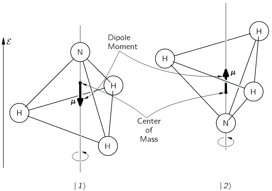
Don’t shy away now. It’s not so difficult. Try to understand. The nitrogen atom (N) in the ammonia molecule (NH₃) can tunnel through the plane of the three hydrogen (H) atoms, so it can be ‘up’ or ‘down’. This ‘up’ or ‘down’ state has nothing to do with the classical or quantum-mechanical notion of spin, which is related to the magnetic moment. Nothing, i.e. nada, niente, rien, nichts! Indeed, it’s much simpler than that. 🙂 The nitrogen atom could be either beneath or, else, above the plane of the hydrogens, as shown above, with ‘beneath’ and ‘above’ being defined in regard to the molecule’s direction of rotation around its axis of symmetry. That’s all. That’s why we prefer simple numbers to denote those two states, instead of the confusing ‘up’ or ‘down’, or ‘↑’ or ‘↓’ symbols. We’ll just call the two states state ‘1’ and state ‘2’ respectively.

Having said that (i.e. having said that you shouldn’t think of spin, which is related to the angular momentum of some (net) electric charge), the NH₃ molecule does have some electric dipole moment, which is denoted by μ in the illustration and which, depending on the state of the molecule (i.e. the nitrogen atom being above or beneath the plane of the hydrogens), changes the total energy of the molecule by an amount that is equal to +με or −με, with ε some external electric field, as illustrated by the ε arrow on the left-hand side of the diagram. [You may think of that arrow as an electric field vector.] This electric field may vary in time and/or in space, but we’ll not worry about that now. In fact, we should first analyze what happens in the absence of an external field, which is what we’ll do now.

The NH₃ molecule will spontaneously transition from an ‘up’ to a ‘down’ state, or from ‘1’ to ‘2’—and vice versa, of course! This spontaneous transition is also modeled as an uncertainty in its energy. Indeed, we say that, even in the absence of an external electric field, there will be two energy levels, rather than one only: E₀ + A and E₀ − A.

We wrote the amplitude to find the molecule in either one of these two states as:

• C₁(t) = 〈 1 | ψ 〉 = (1/2)·e^{−(i/ħ)·(E₀ − A)·t} + (1/2)·e^{−(i/ħ)·(E₀ + A)·t} = e^{−(i/ħ)·E₀·t}·cos[(A/ħ)·t]
• C₂(t) =〈 2 | ψ 〉 = (1/2)·e^{−(i/ħ)·(E₀ − A)·t} – (1/2)·e^{−(i/ħ)·(E₀ + A)·t} = i·e^{−(i/ħ)·E₀·t}·sin[(A/ħ)·t]

[Remember: the sum of complex conjugates, i.e e^iθ + e^−iθ reduces to 2·cosθ, while e^iθ − e^−iθ reduces to 2·i·sinθ.]

That gave us the following probabilities:

• P₁ = |C₁|² = cos²[(A/ħ)·t]
• P₂ = |C₂|² = sin²[(A/ħ)·t]

[Remember: the absolute square of i is |i|² = +√1² = +1, so the i in the C₂(t) formula disappears.]

The graph below shows how these probabilities evolve over time. Note that, because of the square, the period of cos²[(A/ħ)·t] and sin²[(A/ħ)·t] is equal to π, instead of the usual 2π.

The interpretation of this is easy enough: if our molecule can be in two states only, and it starts off in one, then the probability that it will remain in that state will gradually decline, while the probability that it flips into the other state will gradually increase. As Feynman puts it: the first state ‘dumps’ probability into the second state as time goes by, and vice versa, so the probability sloshes back and forth between the two states.

The graph above measures time in units of ħ/A but, frankly, the ‘natural’ unit of time would usually be the period, which you can easily calculate as (A/ħ)·T = π ⇔ T = π·ħ/A. In any case, you can go from one unit to another by dividing or multiplying by π. Of course, the period is the reciprocal of the frequency and so we can calculate the molecular transition frequency f₀ as f₀ = A/[π·ħ] = 2A/h. [Remember: h = 2π·ħ, so A/[π·ħ] = 2A/h].

Of course, by now we’re used to using angular frequencies, and so we’d rather write: ω₀ = 2π·f₀ = f₀ = 2π·A/[π·ħ] = 2A/ħ. And because it’s always good to have some idea of the actual numbers – as we’re supposed to model something real, after all – I’ll give them to you straight away. The separation between the two energy levels E₀ + A and E₀ − A has been measured as being equal to 2A = hf₀ ≈ 10⁻⁴ eV, more or less. 🙂 That’s tiny. To avoid having to convert this to joule, i.e. the SI unit for energy, we can calculate the corresponding frequency using h expressed in eV·s, rather than in J·s. We get: f₀ = 2A/h = (1×10⁻⁴ eV)/(4×10⁻¹⁵ eV·s) = 25 GHz. Now, we’ve rounded the numbers here: the exact frequency is 23.79 GHz, which corresponds to microwave radiation with a wavelength of λ = c/f₀ = 1.26 cm.

How does one measure that? It’s simple: ammonia absorbs light of this frequency. The frequency is also referred to as a resonance frequency, as light of this frequency, i.e. microwave radiation, will also induce transitions from one state to another. In fact, that’s what the stimulated emission of radiation principle is all about. But we’re getting ahead of ourselves here. It’s time to look at what happens if we do apply some external electric field, which is what we’ll do now.

Polarization and induced transitions

As mentioned above, an electric field will change the total energy of the molecule by an amount that is equal to +με or −με. Of course, the plus or the minus in front of με depends both on the direction of the electric field ε, as well as on the direction of μ. However, it’s not like our molecule might be in four possible states. No. We assume the direction of the field is given, and then we have two states only, with the following energy levels:

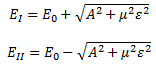
Don’t rack your brain over how you get that square root thing. You get it when applying the general solution of a pair of Hamiltonian equations to this particular case. For full details on how to get this general solution, I’ll refer you to Feynman. Of course, we’re talking base states here, which do not always have a physical meaning. However, in this case, they do: a jet of ammonia gas will split in an inhomogeneous electric field, and it will split according to these two states, just like a beam of particles with different spin in a Stern-Gerlach apparatus. A Stern-Gerlach apparatus splits particle beams because of an inhomogeneous magnetic field, however. So here we’re talking an electric field.

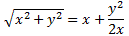
It’s important to note that the field should not be homogeneous, for the very same reason as to why the magnetic field in the Stern-Gerlach apparatus should not be homogeneous: it’s because the force on the molecules will be proportional to the derivative of the energy. So if the energy doesn’t vary—so if there is no strong field gradient—then there will be no force. [If you want to get more detail, check the section on the Stern-Gerlach apparatus in my post on spin and angular momentum.] To be precise, if με is much smaller than A, then one can use the following approximation for the square root in the expressions above:

The energy expressions then reduce to: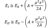

And then we can calculate the force on the molecules as:

The bottom line is that our ammonia jet will split into two separate beams: all molecules in state I will be deflected toward the region of lower ε², and all molecules in state II will be deflected toward the region of larger ε². [We talk about ε² rather than ε because of the ∇ε² gradient in that force formula. However, you could, of course, simplify and write ∇ε² as ∇ε² = 2ε∇ε.] So, to make a long story short, we should now understand the left-hand side of the schematic maser diagram below. It’s easy to understand that the ammonia molecules that go into the maser cavity are polarized.

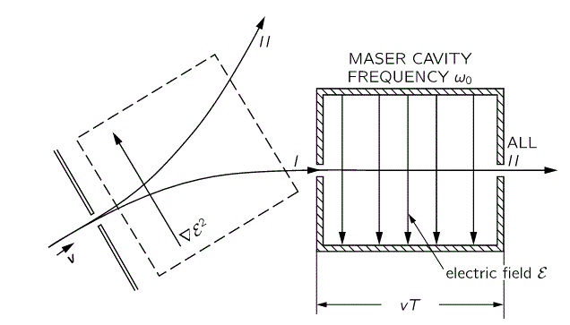
To understand the maser, we need to understand how the maser cavity works. It’s a so-called resonant cavity, and we’ve got an electric field in it as well. The field direction happens to be south as we’re looking at it right now, but in an actual maser we’ll have an electric field that varies sinusoidally. Hence, while the direction of the field is always perpendicular to the direction of motion of our ammonia molecules, it switches from south to north and vice versa all of the time. We write ε as:

ε = 2ε₀cos(ω·t) = ε₀(e^i·ω·t + e^−i·ω·t)

Now, you’ve guessed it, of course. If we ensure that ω = ω₀ = 2A/ħ, then we’ve got a maser. In fact, the result is a similar graph:

Let’s first explain this graph. We’ve got two probabilities here:

• P_I = cos²[(με₀/ħ)·t]
• P_II = sin²[(με₀/ħ)·t]

So that’s just like the P₁ =  cos²[(A/ħ)·t] and P₂ = sin²[(A/ħ)·t] probabilities we found for spontaneous transitions. In fact, the formulas for the related amplitudes are also similar to those for C₁(t) and C₂(t):

• C_I(t) = 〈 I | ψ 〉 = e^{−(i/ħ)·E_I·t}·cos[(με₀/ħ)·t], which is equal to:

C_I(t) = e^{−(i/ħ)·(E₀+A)·t}·cos[(με₀/ħ)·t] = e^{−(i/ħ)·(E₀+A)·t}·(1/2)·[e^{i·(με₀/ħ)·t} + e^{−i·(με₀/ħ)·t}] = (1/2)·e^{−(i/ħ)·(E₀+A−με₀)·t} + (1/2)·e^{−(i/ħ)·(E₀+A+με₀)·t} 

• C_II(t) = 〈 II | ψ 〉 = i·e^{−(i/ħ)·E_II·t}·sin[(με₀/ħ)·t], which is equal to:

 C_II(t) = e^{−(i/ħ)·(E₀−A)·t}·i·sin[(με₀/ħ)·t] = e^{−(i/ħ)·(E₀−A)·t}·(1/2)·[e^{i·(με₀/ħ)·t} − e^{−i·(με₀/ħ)·t}] = (1/2)·e^{−(i/ħ)·(E₀−A−με₀)·t} – (1/2)·e^{−(i/ħ)·(E₀−A+με₀)·t} 

But so here we are talking induced transitions. As you can see, the frequency and, hence, the period, depend on the strength, or magnitude, of the electric field, i.e. the ε₀ constant in the ε = 2ε₀cos(ω·t) expression. The natural unit for measuring time would be the period once again, which we can easily calculate as (με₀/ħ)·T = π ⇔ T = π·ħ/με₀. However, Feynman adds an 1/2 factor so as to ensure it’s the time that corresponds to the time a molecule needs to go through the cavity. Well… That’s what he says, at least. I’ll show he’s actually wrong, but the idea is OK.

First have a look at the diagram of our maser once again. You can see that all molecules come in in state I, but are supposed to leave in state II. Now, Feynman says that’s because the cavity is just long enough so as to more or less ensure that all ammonia molecules switch from state I to state II. Hmm… Let’s have a close look at that. What the functions and the graph are telling us is that, at the point t = 1 (with t being measured in those π·ħ/2με₀ units), the probability of being in state I has all been ‘dumped’ into the probability of being in state II! 

So… Well… Our molecules had better be in that state then! 🙂 Of course, the idea is that, as they transition from state I to state II, they lose energy. To be precise, according to our expressions for E_I and E_II above, the difference between the energy levels that are associated with these two states is equal to 2A + μ²ε₀²/A.

Now, a resonant cavity is a cavity designed to keep electromagnetic waves like the oscillating field that we’re talking about here going with minimal energy loss. Indeed, a microwave cavity – which is what we’re having here – is similar to a resonant circuit, except that it’s much better than any equivalent electric circuit you’d try to build, using inductors and capacitors. ‘Much better’ means it hardly needs energy to keep it going. We express that using the so-called Q-factor (believe it or not: the ‘Q’ stands for quality). The Q factor of a resonant cavity is of the order of 10⁶, as compared to 10² for electric circuits that are designed for the same frequencies. But let’s not get into the technicalities here. Let me quote Feynman as he summarizes the operation of the maser:

“The molecule enters the cavity, [and then] the cavity field—oscillating at exactly the right frequency—induces transitions from the upper to the lower state, and the energy released is fed into the oscillating field. In an operating maser the molecules deliver enough energy to maintain the cavity oscillations—not only providing enough power to make up for the cavity losses but even providing small amounts of excess power that can be drawn from the cavity. Thus, the molecular energy is converted into the energy of an external electromagnetic field.”

As Feynman notes, it is not so simple to explain how exactly the energy of the molecules is being fed into the oscillations of the cavity: it would require to also deal with the quantum mechanics of the field in the cavity, in addition to the quantum mechanics of our molecule. So we won’t get into that nitty-gritty—not here at least. So… Well… That’s it, really.

Of course, you’ll wonder about the orders of magnitude, or minitude, involved. And… Well… That’s where this analysis is somewhat tricky. Let me first say something more about those resonant cavities because, while that’s quite straightforward, you may wonder if they could actually build something like that in the 1950s. 🙂 The condition is that the cavity length must be an integer multiple of the half-wavelength at resonance. We’ve talked about this before. [See, for example, my post on wave modes. More formally, the condition for resonance in a resonator is that the round trip distance, 2·d, is equal to an integral number of the wavelength λ, so we write: 2·d = N·λ, with N = 1, 2, 3, etc. Then, if the velocity of our wave is equal to c, then the resonant frequencies f will be equal to f = (N·c)/(2·d).

Does that makes sense? Of course. We’re talking the speed of light, but we’re also talking microwaves. To be specific, we’re talking a frequency of 23.79 GHz and, more importantly, a wavelength that’s equal to λ = c/f₀ = 1.26 cm, so for the first normal mode (N = 1), we get 2·d = λ ⇔ d = λ/2 = 63 mm. In short, we’re surely not talking nanotechnology here! In other words, the technological difficulties involved in building the apparatus were not insurmountable. 🙂

But what about the time that’s needed to travel through it? What about that length? Now, that depends on the με₀ quantity if we are to believe Feynman here. Now, we actually don’t need to know the actual values for μ or ε₀ : we said that the value of the με₀ product is (much) smaller than the value of A. Indeed, the fields that are used in those masers aren’t all that strong, and the electric dipole moment μ is pretty tiny. So let’s say με₀ = A/2, which is the upper limit for our approximation of that square root above, so 2με₀ = A = 0.5×10⁻⁴ eV. [The approximation for that square root expression is only used when y ≤ x/2.]

Let’s now think about the time. It was measured in units equal to T = π·ħ/2με₀. So our T here is not the T we defined above, which was the period. Here it’s the period divided by two. First the dimensions: ħ is expressed in eV·s, and με₀ is an energy, so we can express it in eV too: 1 eV ≈ 1.6×10⁻¹⁹ J, i.e. 160 zeptojoules. 🙂 π is just a real number, so our T = π·ħ/2με₀ gives us seconds alright. So we get:

T ≈ (3.14×6.6×10⁻¹⁶ eV·s)/(0.5×10⁻⁴ eV) ≈ 40×10⁻¹² seconds

[…] Hmm… That doesn’t look good. Even when traveling at the speed of light – which our ammonia molecule surely doesn’t do! – it would only travel over a distance equal to (3×10⁸ m/s)·(20×10⁻¹² s) = 60×10⁻⁴ m = 0.6 cm = 6 mm. The speed of our ammonia molecule is likely to be only a fraction of the speed of light, so we’d have an extremely short cavity then. The time mentioned is also not in line with what Feynman mentions about the ammonia molecule being in the cavity for a ‘reasonable length of time, say for one millisecond.‘ One millisecond is also more in line with the actual dimensions of the cavity which, as you can see from the historical illustration below, is quite long indeed.

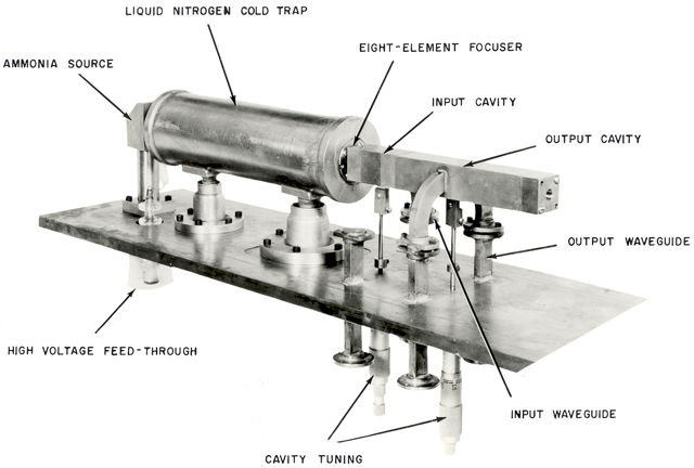
So what’s going on here? Feynman’s statement that T is “the time that it takes the molecule to go through the cavity” cannot be right. Let’s do some good thinking here. For example, let’s calculate the time that’s needed for a spontaneous state transition and compare with the time we calculated above. From the graph and the formulas above, we know we can calculate that from the (A/ħ)·T = π/2 equation. [Note the added 1/2 factor, because we’re not going through a full probability cycle: we’re going through a half-cycle only.] So that’s equivalent to T = (π·ħ)/(2A). We get:

T ≈ (3.14×6.6×10⁻¹⁶ eV·s)/(1×10⁻⁴ eV) ≈ 20×10⁻¹² seconds

The T = π·ħ/2με₀ and T = (π·ħ)/(2A) expression make it obvious that the expected, average, or mean time for a spontaneous versus an induced transition depends on A and με respectively. Let’s be systematic now, so we’ll distinguish T_induced = (π·ħ)/(2με₀) from T_spontaneous = (π·ħ)/(2A) respectively. Taking the ratio, we find:

T_induced/T_spontaneous = [(π·ħ)/(2με₀)]/[(π·ħ)/(2A)] = A/με₀

However, we know the A/με₀ ratio is greater than one, so T_induced/T_spontaneous is greater than one, which, in turn, means that the presence of our electric field – which, let me remind you, dances to the beat of the resonant frequency – causes a slower transition than we would have had if the oscillating electric field were not present. We may write the equation above as:

T_induced = [A/με₀]·T_spontaneous = [A/με₀]·(π·ħ)/(2A) = h/(4με₀)

However, that doesn’t tell us anything new. It just says that the transition period (T) is inversely proportional to the strength of the field (as measured by ε₀). So a weak field will make for a longer transition period (T), with T → ∞ as ε₀ → 0. So it all makes sense, but what do we do with this?

The T_induced/T_spontaneous = [με₀/A]⁻¹ is the most telling. It says that the T_induced/T_spontaneous is inversely proportional to the με₀/A ratio. For example, if the energy με₀ is only one fifth of the energy A, then the time for the induced transition will be five times that of a spontaneous transition. To get something like a millisecond, however, we’d need the με₀/A ratio to go down to like a billionth or something, which doesn’t make sense.

So what’s the explanation? Is Feynman hiding something from us? He’s obviously aware of these periods because, when discussing the so-called three-state maser, he notes that “The | I 〉 state has a long lifetime, so its population can be increased.” But… Well… That’s just not relevant here. He just made a mistake: the length of the maser has nothing to do with it. The thing is: once the molecule transitions from state I to state II, then that’s basically the end of the story as far as the maser operation is concerned. By transitioning, it dumps that energy 2A + μ²ε₀²/A into the electric field, and that’s it. That’s energy that came from outside, because the ammonia molecules were selected so as to ensure they were in state I. So all the transitions afterwards don’t really matter: the ammonia molecules involved will absorb energy as they transition, and then give it back as they transition again, and so on and so on. But that’s no extra energy, i.e. no new or outside energy: it’s just energy going back and forth from the field to the molecules and vice versa.

So, in a way, those P_I and P_II curves become irrelevant. Think of it: the energy that’s related to A and με₀ is defined with respect to a certain orientation of the molecule as well as with respect to the direction of the electric field before it enters the apparatus, and the induced transition is to happen when the electric field inside of the cavity points south, as shown in the diagram. But then the transition happens, and that’s the end of the story, really. Our molecule is then in state II, and will oscillate between state II and I, and back again, and so on and so on, but it doesn’t mean anything anymore, as these flip-flops do not add any net energy to the system as a whole.

So that’s the crux of the matter, really. Mind you: the energy coming out of the first masers was of the order of one microwatt, i.e. 10⁻⁶ joule per second. Not a lot, but it’s something, and so you need to explain it from an ‘energy conservation’ perspective: it’s energy that came in with the molecules as they entered the cavity. So… Well… That’s it.

The obvious question, of course, is: why do we actually need the oscillating field in the cavity? If all molecules come in in the ‘upper’ state, they’ll all dump their energy anyway. Why do we need the field? Well… First, you should note that the whole idea is that our maser keeps going because it uses the energy that the molecules are dumping into its field. The more important thing, however, is that we actually do need the field to induce the transition. That’s obvious from the math. Look at the probability functions once again:

• P_I = cos²[(με₀/ħ)·t]
• P_II = sin²[(με₀/ħ)·t]

If there would be no electric field, i.e. if ε₀ = 0, then P_I = 1 and P_II = 0. So, our ammonia molecules enter in state I and, more importantly, stay in state I forever, so there’s no chance whatsoever to transition to state II. Also note what I wrote above: T_induced = h/(4με₀), and, therefore, we find that T → ∞ as ε₀ → 0.

So… Well… That’s it. I know this is not the ‘standard textbook’ explanation of the maser—it surely isn’t Feynman’s! But… Well… Please do let me know what you think about it. What I write above, indicates the analysis is much more complicated than standard textbooks would want it to be.

There’s one more point related to masers that I need to elaborate on, and that’s its use as an ‘atomic’ clock. So let me quickly do that now.

The use of a maser as an ‘atomic’ clock 

In light of the amazing numbers involved – we talked GHz frequencies, and cycles expressed in picoseconds – we may wonder how it’s possible to ‘tune’ the frequency of the field to the ‘natural’ molecular transition frequency. It will be no surprise to hear that it’s actually not straightforward. It’s got to be right: if the frequency of the field, which we’ll denote by ω, is somewhat ‘off’ – significantly different from the molecular transition frequency ω₀ – then the chance of transitioning from state I to state II shrinks significantly, and actually becomes zero for all practical purposes. That basically means that, if the frequency isn’t right, then the presence of the oscillating field doesn’t matter. In fact, the fact that the frequency has got to be right – with tolerances that, as we will see in a moment, are expressed in billionths – is why a maser can be used as an atomic clock.

The graph below illustrates the principle. If ω = ω₀, then the probability that a transition from state I to II will happen is one, so P_I→II(ω)/P_I→II(ω₀) = 1. If it’s slightly off, though, then the ratio decreases quickly, which means that the P_I→II probability goes rapidly down to zero. [There’s secondary and tertiary ‘bumps’ because of interference of amplitudes, but they’re insignificant.] As evidenced from the graph, the cut-off point is ω − ω₀ = 2π/T, which we can re-write as 2π·f − 2π·f₀ = 2π/T, which is equivalent to writing: (f − f₀)/f₀ =   1/(f₀T). Now, we know that f₀ = 23.79 GHz, but what’s T in this expression? Well… This time around it actually is the time that our ammonia molecules spend in the resonant cavity, from going in to going out, which Feynman says is of the order of a millisecond—so that’s much more reasonable that those 40 picoseconds we calculated. So 1/(f₀T) = 1/[23.79×10⁹·1×⁻³] ≈ 0.042×10⁻⁶ = 42×10⁻⁹  , i.e. 42 billionths indeed, which Feynman rounds to “five parts in 10⁸“, i.e. five parts in a hundred million.

In short, the frequency must be ‘just right’, so as to get a significant transition probability and, therefore, get some net energy out of our maser, which, of course, will come out of our cavity as microwave radiation of the same frequency. Now that’s how one the first ‘atomic’ clock was built: the maser was the equivalent of a resonant circuit, and one could keep it going with little energy, because it’s so good as a resonant circuit. However, in order to get some net energy out of the system, in the form of microwave radiation of, yes, the ammonia frequency, the applied frequency had to be exactly right. To be precise, the applied frequency ω has to match the ω₀ frequency, i.e. the molecular resonance frequency, with a precision expressed in billionths. As mentioned above, the power output is very limited, but it’s real: it comes out through the ‘output waveguide’ in the illustration above or, as the Encyclopædia Brittanica puts it: “Output is obtained by allowing some radiation to escape through a small hole in the resonator.” 🙂

In any case, a maser is not build to produce huge amounts of power. On the contrary, the state selector obviously consumes more power than comes out of the cavity, obviously, so it’s not some generator. Its main use nowadays is as a clock indeed, and so it’s that simple really: if there’s no output, then the ‘clock’ doesn’t work.

It’s an interesting topic, but you can read more about it yourself. I’ll just mention that, while the ammonia maser was effectively used as a timekeeping device, the next-generation of atomic clocks was based on the hydrogen maser, which was introduced in 1960. The principle is the same. Let me quote the Encyclopædia Brittanica on it: “Its output is a radio wave, hose frequency of 1,420,405,751.786 hertz (cycles per second) is reproducible with an accuracy of one part in 30 × 10¹². A clock controlled by such a maser would not get out of step more than one second in 100,000 years.”

So… Well… Not bad. 🙂 Of course, one needs another clock to check if one’s clock is still accurate, and so that’s what’s done internationally: national standards agencies in various countries maintain a network of atomic clocks which are intercompared and kept synchronized. So these clocks define a continuous and stable time scale, collectively, which is referred to as the International Atomic Time (TAI, from the French Temps Atomique International).

Well… That’s it for today. I hope you enjoyed it.

Post scriptum: 

When I say the ammonia molecule just dumps that energy 2A + μ²ε₀²/A into the electric field, and that’s “the end of the story”, then I am simplifying, of course. The ammonia molecule still has two energy levels, separated by an energy difference of 2A and, obviously, it keeps its electric dipole moment and so that continues to play as we’ve got an electric field in the cavity. In fact, the ammonia molecule has a high polarizability coefficient, which means it’s highly sensitive to the electric field inside of the cavity. So, yes, the molecules will continue ‘dancing’ to be the beat of the field indeed, and absorbing and releasing energy, in accordance with that 2A and με₀ factor, and so the probability curves do remain relevant—of course! However, we talked net energy going into the field, and so that’s where the ‘end of story’ story comes in. I hope I managed to make that clear.

In fact, there’s lots of other complications as well, and Feynman mentions them briefly in his account of things. But let’s keep things simple here. 🙂 Also, if you’d want to know how we get that P_I→II(ω)/P_I→II(ω₀), check it out in Feynman. However, I have to warn you: the math involved is not easy. Not at all, really. The set of differential equations that’s involved is complicated, and it takes a while to understand why Feynman uses the trial functions he uses. So the solution that comes out, i.e. those simple P_I = cos²[(με₀/ħ)·t] and P_II = sin²[(με₀/ħ)·t] functions, makes sense—but, if you check it out, you’ll see the whole mathematical argument is rather complicated. That’s just how it is, I am afraid. 🙂

Some content on this page was disabled on June 16, 2020 as a result of a DMCA takedown notice from The California Institute of Technology. You can learn more about the DMCA here:

https://wordpress.com/support/copyright-and-the-dmca/
Some content on this page was disabled on June 16, 2020 as a result of a DMCA takedown notice from The California Institute of Technology. You can learn more about the DMCA here:

https://wordpress.com/support/copyright-and-the-dmca/