
Introduction
Every student of physics learns that the magnetic moment of the electron is given, to first approximation, by what is referred to as the Dirac value or – the more commonly used term – the Bohr magneton:
μe = μB = (ħ/2)·(qe/me)
We separate the two factors in it because our (neo-classical) RealQM framework interprets (i) the qe/me factor as a form factor which distinguishes the electron from, say, a proton or the more massive muon-electron (how much charge per mass or energy unit is ‘packed’ into the particle?), and (ii) ħ as the ubiquitous quantum of action that determines how energy, linear or angular momentum, or – in this case – magnetic moments are quantized. Think of it like this: charge comes in lumps (elementary charged particles), and its dynamical properties come in lumps too.
What about the 1/2 factor? We must refer to our Lecture on Quantum Behavior here for a rather common-sense interpretation of the g-factor and the spin-1/2 property of elementary matter-particles. The electron – interpreted as a dynamic oscillation of charge – ‘packs’ one Planck unit of physical action in each cycle of the oscillation but the angular momentum of the orbiting charge only explains half of the energy (and, therefore, the mass of the electron). The other half is in the electromagnetic field it generates, which keeps the charge spinning and effectively explains the magnetic dipole moment. So, just like protons or the more massive muon-electron, the electron can effectively be described as a ‘fermionic’ or ‘spin-1/2’ particle.
So far, so good. Experiments, however, show that the actual (measured) value is slightly larger. The difference is tiny—about one part in a thousand—and is known as the anomaly in the magnetic moment.
Modern physics explains this anomaly through quantum electrodynamics (QED). In that framework, the correction arises from increasingly complicated perturbative calculations involving “loop diagrams.” The first term in the resulting expansion was derived by Julian Schwinger in 1948 and is equal to /2. That is a very elegant expression, and it explains the anomaly for about 100.15%. Two quick notes must be made here:
1. We effectively wrote: 100.15%. Not 99.85%. Why? Because Schwinger’s factor overshoots the anomaly effectively by about 0.15%. To be precise, (μCODATA-μe)/μe = 0.00115965… and CODATA/2 = 0.0011614… The fact that the Schwinger term slightly overshoots the experimentally measured anomaly, explains why the next correction in QED is actually negative: it must bring the theoretical prediction back into agreement with experiment. This sign swap is rather poorly explained in standard textbooks but, in any case, it is any classical or neo-classical interpretation must probably reproduce such sign patterns. However, in our paper – which is just an introduction to our thinking on this – we do not go into that: we basically just explain – using classical arguments – why α and 2 appear so naturally not only in the leading correction but also higher-order corrections to the Dirac value for the electron’s magnetic moment.
2. Note that we take CODATA values here because these reflect (i) the scientific/academic consensus on the measured magnetic moment (as opposed to the theoretical Dirac value) and (ii) the scientific/academic consensus on the value of the fine-structure constant. The 2019 revision of the system of SI units effectively adds an interesting twist to the debate: the fine-structure constant itself is now defined as being co-determined with the electric and magnetic constant, and the standard relative uncertainty of all three constants is, therefore, now exactly the same: 1.610-10, to be precise.
Let us now go back to the main story line. From the above, it is clear that, while the precision of Schwinger’s factor is higher than 0.15% of one part in a thousand (so that’s a precision of 1.5 parts into a million), we still need higher-order corrections. Why? Because measurements are much more accurate than one part into a million, and some theory should explain all significant digits, isn’t it? 🙂
Using the QED/QFT framework, theoretical physicists have currently computed those higher-order corrections up to what is referred to as the ‘five-loop level’ in QED, with astonishing agreement between theory and experiment. The problem with this ‘astonishing agreement’ is its complexity: the calculations become evermore complicated – as evermore degrees of freedom (cf. the increasing number of Feynman diagrams, which illustrate the various ways in which something might happen) explain less and less, as illustrated in the table below.

In a recently revised working paper on ResearchGate, I therefore explore a different question. Instead of asking how the anomaly emerges from perturbative quantum field theory, I ask whether the structure of the leading correction might also admit a classical interpretation. In the next section, we explain the basics of this classical interpretation, which is based on the ring current model of an electron, which was first advanced by Alfred Lauck Parson in 1915 and, as we explain in our paper on the nature of de Broglie’s matter-wave, also naturally explains Schrödinger’s Zitterbewegung theory. In other words, it is a very classical approach. 🙂
The electron ring current model
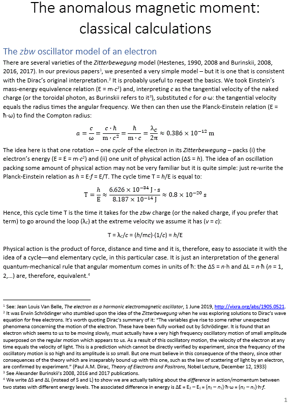
The starting point is, effectively, the old ring-current picture of the electron: imagine a localized “blob” of charge circulating around some center at the speed of light. This blob of charge has no other properties (no rest mass or rest energy) but its charge and, yes, some non-finite size. To be precise, from scattering experiments and the formulas that describe photon-electron scattering, we assume its size is of the order of the classical electron radius. As for the assumption of lightspeed, it is only logical to assume that anything with zero rest mass must travel at lightspeed because the slightest force on it will accelerate it to lightspeed.
When we apply this idea to the electron charge, we must conclude that the radius of this orbital motion will be the Compton radius of the electron. Indeed, when we think of the (elementary) wavefunction r = ψ = a·eiθ as representing the physical position of a pointlike elementary charge – pointlike but not dimensionless – moving at the speed of light around the center of its motion in a space, we must conclude that the radius of this orbital motion – which effectively doubles up as the amplitude of the wavefunction – must be equal to the electron’s Compton radius a = ħ/mc. This can easily be derived from (i) Einstein’s mass-energy equivalence relation, (ii) the Planck-Einstein relation, and (iii) the formula for a tangential velocity:

This electron model also naturally yields the Dirac magnetic moment: we can just calculate it using the standard formula for the magnetic moment of a ring current.
The next step, then, is to acknowledge that charge cannot literally be pointlike. If the circulating charge has a finite spatial extent—of order the classical electron radius—then the current distribution is slightly modified. The mathematical and physical elegance of Schwinger’s factor can then easily be explained by:
(i) noting that the classical electron radius is times the Compton radius of the electron ħ/mec = ħc/Ee, which – in all mainstream accounts of photon-electron scattering experiments – is the scale at which the (free) electron can be localized in a particle-like sense (for more precise academic references (we like LeClair’s (2019) straightforward derivation and textbook explanation of Compton scattering), see our paper on de Broglie’s matter-wave); and
(ii) noting that the 2 factor points at orbital rather than linear motion. Indeed, a division by 2 is all what we need to do whenever we want to relate an orbital velocity or length (a linear wavelength or, when orbital motion rather than linear motion is involved, which is the case here) to radians rather than the SI unit for distance. More generally speaking, the factor pops up whenever we evaluate some loop integral (i.e, whenever we integrate some quantity over a closed orbit using the phase of the (orbital) oscillation).
This strongly suggests that – from the various physical relations in which the fine-structure constant pops up – we should explore its meaning as a scaling constant. More in particular, the fine-structure constant here is the ratio which relates the classical electron radius and the Compton radius. We do not want to distract the reader too much but it is probably good to immediately point out that this interpretation of the fine-structure constant as a geometric ratio is also valid when examining the relation between the Compton radius (free electron) and the Bohr radius (the radius of the negative charge as it manifest itself in a hydrogen atom):
re = α·rC ( 2.81810-15 m), rB = rC/α ( 0.52910-10 m), and rC = ħ/mec = = ħc/Ee ( 386.5310-15 m)
This is intriguing because it shows a 1: 1/α : 1/α2 ‘ladder’ or ‘series’ for the value of (i) what we think of the radius of the elementary charge, (ii) the radius of the elementary particle (free electron) in which this charge manifests itself, and (iii) the interaction radius of the bound electron in its most basic state (i.e., bound by a proton in the hydrogen atom). Needless to say, the multitude of physical phenomena in which the fine-structure constant pops up clearly illustrates that measuring its value can be done in a variety of ways. Measuring it through ever more precise measurements of the anomalous magnetic moment is, therefore, just one way to go about it.
To sum it all up, the hypothesis of a pointlike charge with radius re = α·rC is in completely alignment with the suggestion that (i) any first-order correction to the ideal ring current must scale with α and (ii) because the circulating motion is periodic, any cycle-averaged correction would naturally come with a ‘normalization’ over the full () phase of the orbit. Put these ingredients together and one obtains a leading correction with the same structure as Schwinger’s factor:
Δμ/μe ≈ /2
This does not necessarily replace the first-order QED derivation – especially because we should note that first-order QED calculations are based on the classical electromagnetic equations anyway – but it suggests that the form of the leading term may reflect a simple geometric fact: a finite electromagnetic structure (the ‘naked charge’ inside of a electron, as we call it) undergoing coherent circular motion.
The question, of course, then becomes: what about the higher-order corrections? What geometric or other common-sense arguments could one advance to explain second- or third-order scaling with α. In other words, why would terms with α2 or α3 – or, more generally, (/2)2n – pop up in any theoretical series of powers of α explaining the measured anomaly in the magnetic dipole moment of the electron?
That is what we are discussing in our paper, which we summarize and also comment on this blog post.
Again: why worry about an imprecision of about 1.5 parts in a million?
Again, the casual amateur physics may be tempted to let go of these discussions. The anomaly itself is tiny. The Dirac value already gets the magnetic moment right to about 0.1%, and the famous Schwinger correction then explains almost all of that 1% (about 100.15%, as we wrote). So, the higher-order QED terms only account for a very tiny fraction of the anomaly: something like 0.00015% (so that’s 1.5 parts in a million, indeed). So, why should we look for alternative or more comprehensive interpretations?
The answer is this: because the anomalous magnetic moment is one of the most precise measurements in all of science. Therefore, understanding why i) its leading structure has the form (/2 but (2) at the same time, why this leading structure does not fully explain the measured anomaly is not merely a numerical curiosity. It should tell us something about the underlying geometry of electromagnetic interactions. In other words, the tiny discrepancy carries a lot of conceptual weight.
This ‘conceptual weight’ may be illustrated by noting the complexities in QED/QFT calculations. They seem to contradict Occam’s Razor Principle: evermore complicated calculations – which result from allowing evermore degrees of freedom in the higher-order analysis, as illustrated in the table above – seem to explain less and less.
That is probably one of the reasons why there is discontent with the approach even in mainstream academics. We will let the reader google this – we warmly recommend Google’s Gemini assistant in this regard – but, as an example, it looks like lattice theory is currently rapidly emerging as a strong non-perturbative approach to ‘explaining’ the anomaly. [We put ‘explaining’ in brackets because, as far as we can see, lattice theory is, just like QED/QFT a predominantly mathematical approach, in the sense that its first principles are mathematical principles rather than physical laws). Below we briefly highlight this competing approach within the so-called Standard Model, which makes one wonder if there is still a thing such as a ‘standard’ model for explaining physics.
- Perturbative QED: Treats interactions as small corrections (powers of the fine-structure constant) using Feynman diagrams. This works for the electron because its coupling is weak, but the complexity grows exponentially at higher orders.
- Lattice Theory: Discretizes spacetime into a 4D grid (lattice) of points. It calculates interactions directly from first principles using Monte Carlo simulations on supercomputers, rather than summing infinite series of diagrams.
We must also note to another scientific breakthrough which, in our not-so-humble view, has received insufficient attention, and that is the 2019 revision of SI units. Let us discuss the most salient points of this very significant scientific revision.
The fine-structure constant and the 2019 revision of SI units
The extraordinary precision of the anomaly measurement is very closely connected to the discussion on (i) what the fine-structure constant α. actually is or represents in physics (as mentioned above, it pops up in many relations and equations) and, accordingly, (ii) how we should measure it.
Historically, α was measured through a variety of experiments and then used as an input for theoretical calculations. QED/QFT may be said to have inversed that logic: the measurement of the electron’s anomalous magnetic moment are used to then insert it the QED expansion, which is then used to solve for α. The result is, effectively, one of the most precise determinations of the fine-structure constant currently available but, to me, it looks like the 2019 revision of the SI system changed the conceptual landscape. Indeed, the 2019 revision of SI units clearly implies that (i) the fine-structure constant, (ii) the electric constant, and (iii) the magnetic constant must be co-determined because of the following physical equations:

Hence, the 2019 revision of SI units – which, we think, incorporates all of physics – makes it clear that, unlike precisely defined units such as the meter, second, charge, or exactly defined constants of Nature – such as the speed of light, charge, and the quantum of action – neither of these three constants of Nature (electric constant, magnetic constant, and fine-structure constant) have exact values: they must, effectively, be measured in physical experiments and, importantly, their values must be co-determined in such experiments. Indeed, the relations above imply that the relative standard uncertainty in the measures for all three constants, which is currently at 1.610-10, must remain the same in order to ensure conceptual agreement between experiment and theory.
We will not dwell too long on this because we ourselves still need to think through this some more. However, what we write above makes it obvious that this is very important when considering claims about the precision of both the experimental data as well as theoretical arguments on the anomaly: the precision is, indeed, extraordinary – and will probably become even more extraordinary over the coming decades – but, when evaluating any theoretical model explaining this anomaly, it is obvious such theory can no longer be viewed in isolation. Other physical interpretations of the fine-structure constant – such as the geometric interpretation we advance here – must also be considered.
Note: The above probably explains why CODATA remains rather conservative (as compared to the precision of experimental measurements, that is) in its consensus value for the fine-structure constant and the two electromagnetic constants: their value only has roughly ten significant digits. That is about 10000 times better than one part in a million but, still, it effectively does not quite reflect the accuracy of modern-day experiments. Instead, this standard relative uncertainty now probably reflects both theoretical as well as experimental uncertainties, and the theoretical uncertainties should, in our not-so-humble view, also include a critical analysis of the modern-day QED/QFT framework.
Classical or neo-classical explanations of higher-order terms
Again, the aim of our paper is not to fundamentally question or replace quantum electrodynamics, which seems to remain one of the most successful theories ever constructed. Rather, it is to ask whether the leading structure and higher-order corrections in the mainstream explanation of the anomalous magnetic moment might also admit a complementary geometric or other more fundamental interpretation. We think it does. Let us list all obvious elements of such more fundamental interpretation:
1. The Bohr magneton or Dirac’s formula for the magnetic dipole moment emerges naturally from the age-old electron ring current model, which was first advanced by Alfred Lauck Parson in 1915 and, as we explain in our paper on the nature of de Broglie’s matter-wave, also naturally explains Schrödinger’s Zitterbewegung theory.
2. The first-order correction (Schwinger’s factor) emerges, equally naturally, from the assumption that something that is infinitesimally small (i.e, something with zero physical size) does not exist and, hence, that (i) charge must have some size, and (ii) that, for an electron, this size is given by the classical electron radius. The inuuition here was explained above, and the detail of it is described in the paper we want to promote here. [You would not expect us to just copy-paste our paper in a blog article, isn’t it? :-)]
3. To explain the necessity and/or emergence of second- and higher-order terms, we think of the following:
(i) The assumption of an oscillation naked charge – whose size is not infinitesimally small but of the order of the classical electron radius – inside of the electron naturally leads to what we refer to as ‘finite-size’ corrections to the Compton radius. These corrections probably scale just like α but, when allowing for more advanced ideas such as self-interaction (we admit that we are not a fan but, when everything is said and done, self-interaction is an idea which the classical physicists did like to explore), may also be linear in α2, α3 or higher-order terms.
(ii) Intrinsic spin is, of course, a very obvious candidate for a correction of the core Dirac value of the magnetic moment of an electron. Indeed, if one thinks of the electron as an oscillation of some naked charge, then this small charge distribution itself should make one rotation around its own axis as it orbits around the center of the electron and, hence, this must result in a combined magnetic dipole moment that is slightly different from the Bohr magneton. We asked AI (ChatGPT) to do a quick calculation and – using the standard formula for the magnetic moment of a uniformly charged solid sphere of radius re rotating around its own axis with the same angular velocity ω as its orbital motion – the ratio of (1) this intrinsic magnetic moment and (2) the orbital magnetic moment (i.e., the Bohr magneton) should equal 4α2/5. In other words, this intrinsic spin effects enters at order α². Hence, this is structurally consistent with the observed perturbative hierarchy, in which the leading correction is proportional to α, and higher-order corrections scale with higher powers.
In our paper, we refer to the above alternative explanations as the ‘finite-size’ and ‘intrinsic dipole’ contributions to the magnetic moment, respectively, and we treat them in one and the same chapter because, as mentioned, they are prime candidates for the first- and second-order corrections to the theoretical magnetic moment of the electron.
As for higher-order corrections, we worked with AI to identify a number of additional candidate explanations. Frankly, these convince us somewhat less than the obvious theoretical remarks above but they cannot be dismissed out of hand. We, therefore, list and detail these in a separate chapter in the paper. They include explorations of:
(iii) The precessional motion of the presumed blob of charge in the electron, which one would expect it to have as a result of its intrinsic spin: such and like effects may also be referred to as projection effects resulting from the fact that, in real-life experiments, the free electron is being contained in a Penning trap by an electromagnetic field with which it obviously interacts. The measurement, therefore, must take into account various additional motions – such as complicated precessional or nutational motion – which, again, we will just categorize under the category of ‘projection effects’. [We recommend the reader to dive into the intricacies of what a Penning trap actually is, and look at the amazing technologies involved: a Penning trap combines (i) a homogeneous, strong axial magnetic field for radial confinement as well as (ii) an electrostatic quadrupole field to provide axial confinement.]
(iv) Various interactions which may be categorized as presumed classical ‘self-interaction’ effects. Such effects include interactions between presumed charge elements within the blob, or between the blob and the electromagnetic field sustaining its motion. However, we intuitively feel one can think of many self-interaction effects and, therefore, these theoretical candidate contributions feel quite ad hoc.
(v) Finally, ChatGPT also alludes to complicated corrections that might or should be made as a result of the cycle-averaging or dynamical smearing which is inherent to the ring current model. Indeed, we treat a continuous current distribution just the same as a localized charge in some regular orbital motion. While one might argue we are looking at scales here at which Maxwell’s equations combined with the Planck-Einstein relation might not make sense and that, therefore, cycle-averaging may not be quite legitimate, we are less convinced.
We will end our list here and make two important remarks:
1. From what we write above, it is obvious that the list of classical or neo-classical explanations is sufficiently rich to justify trying non-perturbative theoretical approaches to solve the so-called mystery of the anomaly.
2. That being said, it is not an infinite list (we only have about five items above) and, as mentioned, some explanations make more sense than others. It is, therefore, most likely that the ultimate classical or neo-classical explanation of the anomaly will not be some wonderfully elegant infinite power series. It will likely be a finite series of common-sense terms – each of which embedding one aspect of a system which, in contrast to what is assumed in QED, has very limited degrees of freedom. As such, it should respect Occam’s Razor Principle: the mathematical expression of the explanation should not be more complicated than the physical situation itself.
[…] So, that’s it for this blog. We let AI re-read this blog post, and write the conclusion. We hope it will encourage you to read the full paper itself.
Conclusion
If this exercise shows anything, it is that the fine-structure constant quietly connects several of the most important length scales in electron physics. The classical electron radius, the Compton radius, and the Bohr radius form a simple ladder separated by powers of α. That pattern appears so often in electron physics that it is difficult to believe it is merely accidental.
The ring-current model explored in the working paper uses this observation as a starting point. Once the electron is viewed as a localized charge distribution undergoing coherent circular motion, the Dirac magnetic moment emerges naturally from classical electromagnetism. Introducing a finite charge size of order the classical electron radius then leads to corrections that scale with the ratio (re/rC= α). Because the motion is periodic, these corrections are naturally normalized over all phases within a cycle (2), yielding a leading contribution with the same structure as Schwinger’s famous factor.
Whether this geometric interpretation ultimately captures part of the real physical mechanism behind the anomaly remains an open question. What the present work suggests, however, is that the leading structure of the anomalous magnetic moment may not be as mysterious as it sometimes appears. It may reflect a simple interplay between electromagnetic length scales and the geometry of circular motion.
The purpose of this investigation is therefore not to challenge the extraordinary success of quantum electrodynamics. Rather, it is to ask whether the hierarchy of corrections normally obtained through perturbative calculations might also admit a complementary physical interpretation. If the electron is indeed a finite electromagnetic structure rather than an abstract point particle, then at least some features of the anomaly might ultimately have a geometric explanation.
Even if this line of reasoning proves incomplete, it highlights an intriguing fact: the fine-structure constant continues to appear as a scaling parameter linking the structure of the electron to the structure of atoms. Understanding why those scales are related the way they are may still teach us something fundamental about the organization of electromagnetic phenomena.
The full working paper can be found here. As always, comments, questions, and critical feedback are very welcome.

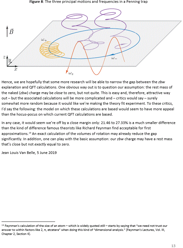
 Let us now look at the other frequency fs. It is the Larmor or precession frequency. It is (also) a classical thing: if we think of the electron as a tiny magnet with a magnetic moment that is proportional to its angular momentum, then it should, effectively, precess in a magnetic field. The analysis of precession is quite straightforward. The geometry of the situation is shown below and we may refer to (almost) any standard physics textbook for the derivation.
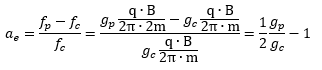 Hence, the so-called anomalous magnetic moment of an electron is nothing but the ratio of two mathematical factors – definitions, basically – which we can express in terms of actual frequencies:
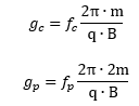 Our formula for ae now becomes:
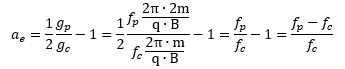 Of course, if we use the μ/J = 2m/q equality, then the fp/fc ratio will be equal to 1/2, and ae will not be zero but −1/2:
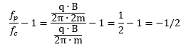 However, as mentioned above, we should not do that. The precession causes the magnetic moment and the angular momentum to wobble. Hence, there is nothing anomalous about the anomalous magnetic moment. We should not wonder why its value is not zero. We should wonder why it is so nearly zero.