I am of the opinion that Richard Feynman’s wonderful little common-sense introduction to the ‘uncommon-sensy‘ theory of quantum electrodynamics (The Strange Theory of Light and Matter), which were published a few years before his death only, should be mandatory reading for high school students.

I actually mean that: it should just be part of the general education of the first 21st century generation. Either that or, else, the Education Board should include a full-fledged introduction to complex analysis and quantum physics in the curriculum. 🙂

Having praised it (just now, as well as in previous posts), I re-read it recently during a trek in Nepal with my kids – I just grabbed the smallest book I could find the morning we left 🙂 – and, frankly, I now think Ralph Leighton, who transcribed and edited these four short lectures, could have cross-referenced it better. Moreover, there are two or three points where Feynman (or Leighton?) may have sacrificed accuracy for readability. Let me recapitulate the key points and try to improve here and there.

Amplitudes and arrows

The booklet avoids scary mathematical terms and formulas but doesn’t avoid the fundamental concepts behind, and it doesn’t avoid the kind of ‘deep’ analysis one needs to get some kind of ‘feel’ for quantum mechanics either. So what are the simplifications?

A probability amplitude (i.e. a complex number) is, quite simply, an arrow, with a direction and a length. Thus Feynman writes: “Arrows representing probabilities from 0% to 16% [as measured by the surface of the square which has the arrow as its side] have lengths from 0 to 0.4.” That makes sense: such geometrical approach does away, for example, with the need to talk about the absolute square (i.e. the square of the absolute value, or the squared norm) of a complex number – which is what we need to calculate probabilities from probability amplitudes. So, yes, it’s a wonderful metaphor. We have arrows and surfaces now, instead of wave functions and absolute squares of complex numbers.

The way he combines these arrows make sense too. He even notes the difference between photons (bosons) and electrons (fermions): for bosons, we just add arrows; for fermions, we need to subtract them (see my post on amplitudes and statistics in this regard).

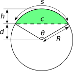
There is also the metaphor for the phase of a wave function, which is a stroke of genius really (I mean it): the direction of the ‘arrow’ is determined by a stopwatch hand, which starts turning when a photon leaves the light source, and stops when it arrives, as shown below.

OK. Enough praise. What are the drawbacks?

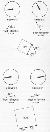
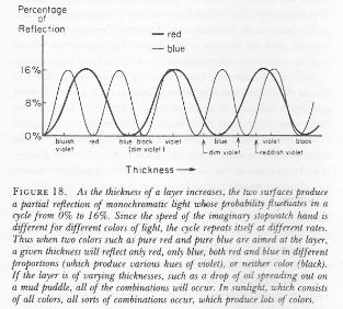
The illustration above accompanies an analysis of how light is either reflected from the front surface of a sheet of a glass or, else, from the back surface. Because it takes more time to bounce off the back surface (the path is associated with a greater distance), the front and back reflection arrows point in different directions indeed (the stopwatch is stopped somewhat later when the photon reflects from the back surface). Hence, the difference in phase (but that’s a term that Feynman also avoids) is determined by the thickness of the glass. Just look at it. In the upper part of the illustration above, the thickness is such that the chance of a photon reflecting off the front or back surface is 5%: we add two arrows, each with a length of 0.2, and then we square the resulting (aka final) arrow. Bingo! We get a surface measuring 0.05, or 5%.

Huh? Yes. Just look at it: if the angle between the two arrows would be 90° exactly, it would be 0.08 or 8%, but the angle is a bit less. In the lower part of the illustration, the thickness of the glass is such that the two arrows ‘line up’ and, hence, they form an arrow that’s twice the length of either arrow alone (0.2 + 0.2 = 0.4), with a square four times as large (0.16 = 16%). So… It all works like a charm, as Feynman puts it.

[…]

But… Hey! Look at the stopwatch for the front reflection arrows in the upper and lower diagram: they point in the opposite direction of the stopwatch hand! Well… Hmm… You’re right. At this point, Feynman just notes that we need an extra rule: “When we are considering the path of a photon bouncing off the front surface of the glass, we reverse the direction of the arrow.”

He doesn’t say why. He just adds this random rule to the other rules – which most readers who read this book already know. But why this new rule? Frankly, this inconsistency – or lack of clarity – would wake me up at night. This is Feynman: there must be a reason. Why?

Initially, I suspected it had something to do with the two types of ‘statistics’ in quantum mechanics (i.e. those different rules for combining amplitudes of bosons and fermions respectively, which I mentioned above). But… No. Photons are bosons anyway, so we surely need to add, not subtract. So what is it?

[…] Feynman explains it later, much later – in the third of the four chapters of this little book, to be precise. It’s, quite simply, the result of the simplified model he uses in that first chapter. The photon can do anything really, and so there are many more arrows than just two. We actually should look at an infinite number of arrows, representing all possible paths in spacetime, and, hence, the two arrows (i.e. the one for the reflection from the front and back surface respectively) are combinations of many other arrows themselves. So how does that work?

An analysis of partial reflection (I)

The analysis in Chapter 3 of the same phenomenon (i.e. partial reflection by glass) is a simplified analysis too, but it’s much better – because there are no ‘random’ rules here. It is what Leighton promises to the reader in his introduction: “A complete description, accurate in every detail, of a framework onto which more advanced concepts can be attached without modification. Nothing has to be ‘unlearned’ later.”

Well… Accurate in every detail? Perhaps not. But it’s good, and I still warmly recommend a reading of this delightful little book to anyone who’d ask me what to read as a non-mathematical introduction to quantum mechanics. I’ll limit myself here to just some annotations.

The first drawing (a) depicts the situation:

1. A photon from a light source is being reflected by the glass. Note that it may also go straight through, but that’s a possibility we’ll analyze separately. We first assume that the photon is effectively being reflected by the glass, and so we want to calculate the probability of that event using all these ‘arrows’, i.e. the underlying probability amplitudes.
2. As for the geometry of the situation: while the light source and the detector seem to be positioned at some angle from the normal, that is not the case: the photon travels straight down (and up again when reflected). It’s just a limitation of the drawing. It doesn’t really matter much for the analysis: we could look at a light beam coming in at some angle, but so we’re not doing that. It’s the simplest situation possible, in terms of experimental set-up that is. I just want to be clear on that.

Now, rather than looking at the front and back surface only (as Feynman does in Chapter 1), the glass sheet is now divided into a number of very thin sections: five, in this case, so we have six points from which the photon can be scattered into the detector at A: X₁ to X₆. So that makes six possible paths. That’s quite a simplification but it’s easy to see it doesn’t matter: adding more sections would result in many more arrows, but these arrows would also be much smaller, and so the final arrow would be the same.

The more significant simplification is that the paths are all straight paths, and that the photon is assumed to travel at the speed of light, always. If you haven’t read the booklet, you’ll say that’s obvious, but it’s not: a photon has an amplitude to go faster or slower than c but, as Feynman points out, these amplitudes cancel out over longer distances. Likewise, a photon can follow any path in space really, including terribly crooked paths, but these paths also cancel out. As Feynman puts it: “Only the paths near the straight-line path have arrows pointing in nearly the same direction, because their timings are nearly the same, and only these arrows are important, because it is from them that we accumulate a large final arrow.” That makes perfect sense, so there’s no problem with the analysis here either.

So let’s have a look at those six arrows in illustration (b). They point in a slightly different direction because the paths are slightly different and, hence, the distances (and, therefore, the timings) are different too. Now, Feynman (but I think it’s Leighton really) loses himself here in a digression on monochromatic light sources. A photon is a photon: it will have some wave function with a phase that varies in time and in space and, hence, illustration (b) makes perfect sense. [I won’t quote what he writes on a ‘monochromatic light source’ because it’s quite confusing and, IMHO, not correct.]

The stopwatch metaphor has only one minor shortcoming: the hand of a stopwatch rotates clockwise (obviously!), while the phase of an actual wave function goes counterclockwise with time. That’s just convention, and I’ll come back to it when I discuss the mathematical representation of the so-called wave function, which gives you these amplitudes. However, it doesn’t change the analysis, because it’s the difference in the phase that matters when combining amplitudes, so the clock can turn in either way indeed, as long as we’re agreed on it.

At this point, I can’t resist: I’ll just throw the math in. If you don’t like it, you can just skip the section that follows.

Feynman’s arrows and the wave function

The mathematical representation of Feynman’s ‘arrows’ is the wave function:

f = f(x–ct)

Is that the wave function? Yes. It is: it’s a function whose argument is x – ct, with x the position in space, and t the time variable. As for c, that’s the speed of light. We throw it in to make the units in which we measure time and position compatible. 

Really? Yes: f is just a regular wave function. To make it look somewhat more impressive, I could use the Greek symbol Φ (phi) or Ψ (psi) for it, but it’s just what it is: a function whose value depends on position and time indeed, so we write f = f(x–ct). Let me explain the minus sign and the c in the argument.

Time and space are interchangeable in the argument, provided we measure time in the ‘right’ units, and so that’s why we multiply the time in seconds with c, so the new unit of time becomes the time that light needs to travel a distance of one meter. That also explains the minus sign in front of ct: if we add one distance unit (i.e. one meter) to the argument, we have to subtract one time unit from it – the new time unit of course, so that’s the time that light needs to travel one meter – in order to get the same value for f. [If you don’t get that x–ct thing, just think a while about this, or make some drawing of a wave function. Also note that the spacetime diagram in illustration (b) above assumes the same: time is measured in an equivalent unit as distance, so the 45% line from the south-west to the north-east, that bounces back to the north-west, represents a photon traveling at speed c in space indeed: one unit of time corresponds to one meter of travel.]

Now I want to be a bit more aggressive. I said f is a simple function. That’s true and not true at the same time. It’s a simple function, but it gives you probability amplitudes, which are complex numbers – and you may think that complex numbers are, perhaps, not so simple. However, you shouldn’t be put off. Complex numbers are really like Feynman’s ‘arrows’ and, hence, fairly simple things indeed. They have two dimensions, so to say: an a– and a b-coordinate. [I’d say an x– and y-coordinate, because that’s what you usually see, but then I used the x symbol already for the position variable in the argument of the function, so you have to switch to a and b for a while now.]

This a– and b-coordinate are referred to as the real and imaginary part of a complex number respectively. The terms ‘real’ and ‘imaginary’ are confusing because both parts are ‘real’ – well… As real as numbers can be, I’d say. 🙂 They’re just two different directions in space: the real axis is the a-axis in coordinate space, and the imaginary axis is the b-axis. So we could write it as an ordered pair of numbers (a, b). However, we usually write it as a number itself, and we distinguish the b-coordinate from the a-coordinate by writing an i in front: (a, b) = a + ib. So our function f = f(x–ct) is a complex-valued function: it will give you two numbers (an a and a b) instead of just one when you ‘feed’ it with specific values for x and t. So we write:

f = f(x–ct) = (a, b) = a + ib

So what’s the shape of this function? Is it linear or irregular or what? We’re talking a very regular wave function here, so it’s shape is ‘regular’ indeed. It’s a periodic function, so it repeats itself again and again. The animations below give you some idea of such ‘regular’ wave functions. Animation A and B shows a real-valued ‘wave’: a ball on a string that goes up and down, for ever and ever. Animations C to H are – believe it or not – basically the same thing, but so we have two numbers going up and down. That’s all.

The wave functions above are, obviously, confined in space, and so the horizontal axis represents the position in space. What we see, then, is how the real and imaginary part of these wave functions varies as time goes by. [Think of the blue graph as the real part, and the imaginary part as the pinkish thing – or the other way around. It doesn’t matter.] Now, our wave function – i.e. the one that Feynman uses to calculate all those probabilities – is even more regular than those shown above: its real part is an ordinary cosine function, and it’s imaginary part is a sine. Let me write this in math:

f = f(x–ct) = a + ib = r(cosφ + isinφ)

It’s really the most regular wave function in the world: the very simple illustration below shows how the two components of f vary as a function in space (i.e. the horizontal axis) while we keep the time fixed, or vice versa: it could also show how the function varies in time at one particular point in space, in which case the horizontal axis would represent the time variable. It is what it is: a sine and a cosine function, with the angle φ as its argument.

Note that a sine function is the same as a cosine function, but it just lags a bit. To be precise, the phase difference is 90°, or π/2 in radians (the radian (i.e. the length of the arc on the unit circle) is a much more natural unit to express angles, as it’s fully compatible with our distance unit and, hence, most – if not all – of our other units). Indeed, you may or may not remember the following trigonometric identities: sinφ = cos(π/2–φ) = cos(φ–π/2).

In any case, now we have some r and φ here, instead of a and b. You probably wonder where I am going with all of this. Where are the x and t variables? Be patient! You’re right. We’ll get there. I have to explain that r and φ first. Together, they are the so-called polar coordinates of Feynman’s ‘arrow’ (i.e. the amplitude). Polar coordinates are just as good as coordinates as these Cartesian coordinates we’re used to (i.e. a and b). It’s just a different coordinate system. The illustration below shows how they are related to each other. If you remember anything from your high school trigonometry course, you’ll immediately agree that a is, obviously, equal to rcosφ, and b is rsinφ, which is what I wrote above. Just as good? Well… The polar coordinate system has some disadvantages (all of those expressions and rules we learned in vector analysis assume rectangular coordinates, and so we should watch out!) but, for our purpose here, polar coordinates are actually easier to work with, so they’re better.

Feynman’s wave function is extremely simple because his ‘arrows’ have a fixed length, just like the stopwatch hand. They’re just turning around and around and around as time goes by. In other words, r is constant and does not depend on position and time. It’s the angle φ that’s turning and turning and turning as the stopwatch ticks while our photon is covering larger and larger distances. Hence, we need to find a formula for φ that makes it explicit how φ changes as a function in spacetime. That φ variable is referred to as the phase of the wave function. That’s a term you’ll encounter frequently and so I had better mention it. In fact, it’s generally used as a synonym for any angle, as you can see from my remark on the phase difference between a sine and cosine function.

So how do we express φ as a function of x and t? That’s where Euler’s formula comes in. Feynman calls it the most remarkable formula in mathematics – our jewel! And he’s probably right: of all the theorems and formulas, I guess this is the one we can’t do without when studying physics. I’ve written about this in another post, and repeating what I wrote there would eat up too much space, so I won’t do it and just give you that formula. A regular complex-valued wave function can be represented as a complex (natural) exponential function, i.e. an exponential function with Euler’s number e (i.e. 2.728…) as the base, and the complex number iφ as the (variable) exponent. Indeed, according to Euler’s formula, we can write:

f = f(x–ct) = a + ib = r(cosφ + isinφ) = r·e^iφ

As I haven’t explained Euler’s formula (you should really have a look at my posts on it), you should just believe me when I say that r·e^iφ is an ‘arrow’ indeed, with length r and angle φ (phi), as illustrated above, with a and b coordinates a = rcosφ and b = rsinφ. What you should be able to do now, is to imagine how that φ angle goes round and round as time goes by, just like Feynman’s ‘arrow’ goes round and round – just like a stopwatch hand indeed, but note our φ angle turns counterclockwise indeed.

Fine, you’ll say – but so we need a mathematical expression, don’t we? Yes,we do. We need to know how that φ angle (i.e. the variable in our r·e^iφ function) changes as a function of x and t indeed. It turns out that the φ in r·e^iφ can be substituted as follows:

r·e^iφ = r·e^i(ωt–kx) = r·e^{–ik(x–ct)}

Huh? Yes. The phase (φ) of the probability amplitude (i.e. the ‘arrow’) is a simple linear function of x and t indeed: φ = ωt–kx = –k(x–ct). What about all these new symbols, k and ω? The ω and k in this equation are the so-called angular frequency and the wave number of the wave. The angular frequency is just the frequency expressed in radians, and you should think of the wave number as the frequency in space. [I could write some more here, but I can’t make it too long, and you can easily look up stuff like this on the Web.] Now, the propagation speed c of the wave is, quite simply, the ratio of these two numbers: c = ω/k. [Again, it’s easy to show how that works, but I won’t do it here.]

Now you know it all, and so it’s time to get back to the lesson.

An analysis of partial reflection (II)

Why did I digress? Well… I think that what I write above makes much more sense than Leighton’s rather convoluted description of a monochromatic light source as he tries to explain those arrows in diagram (b) above. Whatever it is, a monochromatic light source is surely not “a device that has been carefully arranged so that the amplitude for a photon to be emitted at a certain time can be easily calculated.” That’s plain nonsense. Monochromatic light is light of a specific color, so all photons have the same frequency (or, to be precise, their wave functions have all the same well-defined frequency), but these photons are not in phase. Photons are emitted by atoms, as an electron moves from one energy level to the other. Now, when a photon is emitted, what actually happens is that the atom radiates a train of waves only for about 10^–8 sec, so that’s about 10 billionths of a second. After 10^–8 sec, some other atom takes over, and then another atom, and so on. Each atom emits one photon, whose energy is the difference between the two energy levels that the electron is jumping to or from. So the phase of the light that is being emitted can really only stay the same for about 10^–8 sec. Full stop.

Now, what I write above on how atoms actually emit photons is a paraphrase of Feynman’s own words in his much more serious series of Lectures on Mechanics, Radiation and Heat. Therefore, I am pretty sure it’s Leighton who gets somewhat lost when trying to explain what’s happening. It’s not photons that interfere. It’s the probability amplitudes associated with the various paths that a photon can take. To be fully precise, we’re talking the photon here, i.e. the one that ends up in the detector, and so what’s going on is that the photon is interfering with itself. Indeed, that’s exactly what the ‘craziness’ of quantum mechanics is all about: we sent electrons, one by one, through two slits, and we observe an interference pattern. Likewise, we got one photon here, that can go various ways, and it’s those amplitudes that interfere, so… Yes: the photon interferes with itself.

OK. Let’s get back to the lesson and look at diagram (c) now, in which the six arrows are added. As mentioned above, it would not make any difference if we’d divide the glass in 10 or 20 or 1000 or a zillion ‘very thin’ sections: there would be many more arrows, but they would be much smaller ones, and they would cover the same circular segment: its two endpoints would define the same arc, and the same chord on the circle that we can draw when extending that circular segment. Indeed, the six little arrows define a circle, and that’s the key to understanding what happens in the first chapter of Feynman’s QED, where he adds two arrows only, but with a reversal of the direction of the ‘front reflection’ arrow. Here there’s no confusion – Feynman (or Leighton) eloquently describe what they do:

“There is a mathematical trick we can use to get the same answer [i.e. the same final arrow]: Connecting the arrows in order from 1 to 6, we get something like an arc, or part of a circle. The final arrow forms the chord of this arc. If we draw arrows from the center of the ‘circle’ to the tail of arrow 1 and to the head of arrow 6, we get two radii. If the radius arrow from the center to arrow 1 is turned 180° (“subtracted”), then it can be combined with the other radius arrow to give us the same final arrow! That’s what I was doing in the first lecture: these two radii are the two arrows I said represented the ‘front surface’ and ‘back surface’ reflections. They each have the famous length of 0.2.”

That’s what’s shown in part (d) of the illustration above and, in case you’re still wondering what’s going on, the illustration below should help you to make your own drawings now.

So… That explains the phenomenon Feynman wanted to explain, which is a phenomenon that cannot be explained in classical physics. Let me copy the original here:

Partial reflection by glass—a phenomenon that cannot be explained in classical physics? Really?

You’re right to raise an objection: partial reflection by glass can, in fact, be explained by the classical theory of light as an electromagnetic wave. The assumption then is that light is effectively being reflected by both the front and back surface and the reflected waves combine or cancel out (depending on the thickness of the glass and the angle of reflection indeed) to match the observed pattern. In fact, that’s how the phenomenon was explained for hundreds of years! The point to note is that the wave theory of light collapsed as technology advanced, and experiments could be made with very weak light hitting photomultipliers. As Feynman writes: “As the light got dimmer and dimmer, the photomultipliers kept making full-sized clicks—there were just fewer of them. Light behaved as particles!”

The point is that a photon behaves like an electron when going through two slits: it interferes with itself! As Feynman notes, we do not have any ‘common-sense’ theory to explain what’s going on here. We only have quantum mechanics, and quantum mechanics is an “uncommon-sensy” theory: a “strange” or even “absurd” theory, that looks “cockeyed” and incorporates “crazy ideas”. But… It works.

Now that we’re here, I might just as well add a few more paragraphs to fully summarize this lovely publication – if only because summarizing stuff like this helps me to come to terms with understanding things better myself!

Calculating amplitudes: the basic actions

So it all boils down to calculating amplitudes: an event is divided into alternative ways of how the event can happen, and the arrows for each way are ‘added’. Now, every way an event can happen can be further subdivided into successive steps. The amplitudes for these steps are then ‘multiplied’. For example, the amplitude for a photon to go from A to C via B is the ‘product’ of the amplitude to go from A to B and the amplitude to go from B to C.

I marked the terms ‘multiplied’ and ‘product’ with apostrophes, as if to say it’s not a ‘real’ product. But it is an actual multiplication: it’s the product of two complex numbers. Feynman does not explicitly compare this product to other products, such as the dot (•) or cross (×) product of two vectors, but he uses the ∗ symbol for multiplication here, which clearly distinguishes V∗W from V•W or V×W indeed or, more simply, from the product of two ordinary numbers. [Ordinary numbers? Well… With ‘ordinary’ numbers, I mean real numbers, of course, but once you get used to complex numbers, you won’t like that term anymore, because complex numbers start feeling just as ‘real’ as other numbers – especially when you get used to the idea of those complex-valued wave functions underneath reality.]

Now, multiplying complex numbers, or ‘arrows’ using QED’s simpler language, consists of adding their angles and multiplying their lengths. That being said, the arrows here all have a length smaller than one (because their square cannot be larger than one, because that square is a probability, i.e. a (real) number between 0 and 1), Feynman defines successive multiplication as successive ‘shrinks and turns’ of the unit arrow. That all makes sense – very much sense.

But what’s the basic action? As Feynman puts the question: “How far can we push this process of splitting events into simpler and simpler subevents? What are the smallest possible bits and pieces? Is there a limit?” He immediately answers his own question. There are three ‘basic actions’:

1. A photon goes from one point (in spacetime) to another: this amplitude is denoted by P(A to B).
2. An electron goes from one point to another: E(A to B).
3. An electron emits and/or absorbs a photon: this is referred to as a ‘junction’ or a ‘coupling’, and the amplitude for this is denoted by the symbol j, i.e. the so-called junction number.

How do we find the amplitudes for these?

The amplitudes for (1) and (2) are given by a so-called propagator functions, which give you the probability amplitude for a particle to travel from one place to another in a given time indeed, or to travel with a certain energy and momentum. Judging from the Wikipedia article on these functions, the subject-matter is horrendously complicated, and the formulas are too, even if Feynman says it’s ‘very simple’ – for a photon, that is. The key point to note is that any path is possible. Moreover, there are also amplitudes for photons to go faster or slower than the speed of light (c)! However, these amplitudes make smaller contributions, and cancel out over longer distances. The same goes for the crooked paths: the amplitudes cancel each other out as well.

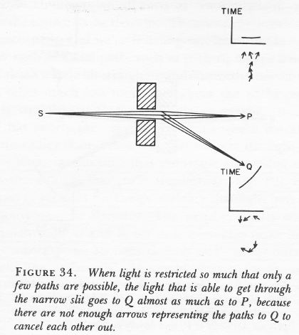
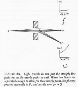
What remains are the ‘nearby paths’. In my previous post (check the section on electromagnetic radiation), I noted that, according to classical wave theory, a light wave does not occupy any physical space: we have electric and magnetic field vectors that oscillate in a direction that’s perpendicular to the direction of propagation, but these do not take up any space. In quantum mechanics, the situation is quite different. As Feynman puts it: “When you try to squeeze light too much [by forcing it to go through a small hole, for example, as illustrated below], it refuses to cooperate and begins to spread out.” He explains this in the text below the second drawing: “There are not enough arrows representing the paths to Q to cancel each other out.”

Not enough arrows? We can subdivide space in as many paths as we want, can’t we? Do probability amplitudes take up space? And now that we’re asking the tougher questions, what’s a ‘small’ hole? What’s ‘small’ and what’s ‘large’ in this funny business?

Unfortunately, there’s not much of an attempt in the booklet to try to answer these questions. One can begin to formulate some kind of answer when doing some more thinking about these wave functions. To be precise, we need to start looking at their wavelength. The frequency of a typical photon (and, hence, of the wave function representing that photon) is astronomically high. For visible light, it’s in the range of 430 to 790 teraherz, i.e. 430–790×10¹² Hz. We can’t imagine such incredible numbers. Because the frequency is so high, the wavelength is unimaginably small. There’s a very simple and straightforward relation between wavelength (λ) and frequency (ν) indeed: c = λν. In words: the speed of a wave is the wavelength (i.e. the distance (in space) of one cycle) times the frequency (i.e. the number of cycles per second). So visible light has a wavelength in the range of 390 to 700 nanometer, i.e. 390–700 billionths of a meter. A meter is a rather large unit, you’ll say, so let me express it differently: it’s less than one thousandth of a micrometer, and a micrometer itself is one thousandth of a millimeter. So, no, we can’t imagine that distance either.

That being said, that wavelength is there, and it does imply that some kind of scale is involved. A wavelength covers one full cycle of the oscillation: it means that, if we travel one wavelength in space, our ‘arrow’ will point in the same direction again. Both drawings above (Figure 33 and 34) suggest the space between the two blocks is less than one wavelength. It’s a bit hard to make sense of the direction of the arrows but note the following:

1. The phase difference between (a) the ‘arrow’ associated with the straight route (i.e. the ‘middle’ path) and (b) the ‘arrow’ associated with the ‘northern’ or ‘southern’ route (i.e. the ‘highest’ and ‘lowest’ path) in Figure 33 is like quarter of a full turn, i.e. 90°. [Note that the arrows for the northern and southern route to P point in the same direction, because they are associated with the same timing. The same is true for the two arrows in-between the northern/southern route and the middle path.]
2. In Figure 34, the phase difference between the longer routes and the straight route is much less, like 10° only.

Now, the calculations involved in these analyses are quite complicated but you can see the explanation makes sense: the gap between the two blocks is much narrower in Figure 34 and, hence, the geometry of the situation does imply that the phase difference between the amplitudes associated with the ‘northern’ and ‘southern’ routes to Q is much smaller than the phase difference between those amplitudes in Figure 33. To be precise,

1. The phase difference between (a) the ‘arrow’ associated with the ‘northern route’ to Q and (b) the ‘arrow’ associated with the ‘southern’ route to Q (i.e. the ‘highest’ and ‘lowest’ path) in Figure 33 is like three quarters of a full turn, i.e. 270°. Hence, the final arrow is very short indeed, which means that the probability of the photon going to Q is very low indeed. [Note that the arrows for the northern and southern route no longer point in the same direction, because they are associated with very different timings: the ‘southern route’ is shorter and, hence, faster.]
2. In Figure 34, we have a phase difference between the shortest and longest route that is like 60° only and, hence, the final arrow is very sizable and, hence, the probability of the photon going to Q is, accordingly, quite substantial.

OK… What did I say here about P(A to B)? Nothing much. I basically complained about the way Feynman (or Leighton, more probably) explained the interference or diffraction phenomenon and tried to do a better job before tacking the subject indeed: how do we get that P(A to B)?

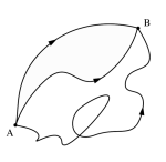
A photon can follow any path from A to B, including the craziest ones (as shown below). Any path? Good players give a billiard ball extra spin that may make the ball move in a curved trajectory, and will also affect its its collision with any other ball – but a trajectory like the one below? Why would a photon suddenly take a sharp turn left, or right, or up, or down? What’s the mechanism here? What are the ‘wheels and gears inside’ of the photon that (a) make a photon choose this path in the first place and (b) allow it to whirl, swirl and twirl like that?

We don’t know. In fact, the question may make no sense, because we don’t know what actually happens when a photon travels through space. We know it leaves as a lump of energy, and we know it arrives as a similar lump of energy. When we actually put a detector to check which path is followed – by putting special detectors at the slits in the famous double-slit experiment, for example – the interference pattern disappears. So… Well… We don’t know how to describe what’s going on: a photon is not a billiard ball, and it’s not a classical electromagnetic wave either. It is neither. The only thing that we know is that we get probabilities that match with the results of experiment if we accept this nonsensical assumptions and do all of the crazy arithmetic involved. Let me get back to the lesson.  

Photons can also travel faster or slower than the speed of light (c is some 3×10⁸ meter per second but, in our special time unit, it’s equal to one). Does that violate relativity? It doesn’t, apparently, but for the reasoning behind I must, once again, refer you to more sophisticated writing.

In any case, if the mathematicians and physicists have to take into account both of these assumptions (any path is possible, and speeds higher or lower than c are possible too!), they must be looking at some kind of horrendous integral, don’t they?

They are. When everything is said and done, that propagator function is some monstrous integral indeed, and I can’t explain it to you in a couple of words – if only because I am struggling with it myself. 🙂 So I will just believe Feynman when he says that, when the mathematicians and physicists are finished with that integral, we do get some simple formula which depends on the value of the so-called spacetime interval between two ‘points’ – let’s just call them 1 and 2 – in space and time. You’ve surely heard about it before: it’s denoted by s² or I (or whatever) and it’s zero if an object moves at the speed of light, which is what light is supposed to do – but so we’re dealing with a different situation here. 🙂 To be precise, I consists of two parts:

1. The distance d between the two points (1 and 2), i.e. Δr, which is just the square root of d² = Δr² = (x₂–x₂)²+(y₂–y₁)²+(z₂–z₁)². [This formula is just a three-dimensional version of the Pythagorean Theorem.]
2. The ‘distance’ (or difference) in time, which is usually expressed in those ‘equivalent’ time units that we introduced above already, i.e. the time that light – traveling at the speed of light 🙂 – needs to travel one meter. We will usually see that component of I in a squared version too: Δt² = (t₂–t₁)², or, if time is expressed in the ‘old’ unit (i.e. seconds), then we write c²Δt² = c²(t₂–t₁)².

Now, the spacetime interval itself is defined as the excess of the squared distance (in space) over the squared time difference:

s² = I = Δr² – Δt² = (x₂–x₂)²+(y₂–y₁)²+(z₂–z₁)² – (t₂–t₁)²

You know we can then define time-like, space-like and light-like intervals, and these, in turn, define the so-called light cone. The spacetime interval can be negative, for example. In that case, Δt² will be greater than Δr², so there is no ‘excess’ of distance over time: it means that the time difference is large enough to allow for a cause–effect relation between the two events, and the interval is said to be time-like. In any case, that’s not the topic of this post, and I am sorry I keep digressing.

The point to note is that the formula for the propagator favors light-like intervals: they are associated with large arrows. Space- and time-like intervals, on the other hand, will contribute much smaller arrows. In addition, the arrows for space- and time-like intervals point in opposite directions, so they will cancel each other out. So, when everything is said and done, over longer distances, light does tend to travel in a straight line and at the speed of light. At least, that’s what Feynman tells us, and I tend to believe him. 🙂

But so where’s the formula? Feynman doesn’t give it, probably because it would indeed confuse us. Just google ‘propagator for a photon’ and you’ll see what I mean. He does integrate the above conclusions in that illustration (b) though. What illustration? 

Oh… Sorry. You probably forgot what I am trying to do here, but so we’re looking at that analysis of partial reflection of light by glass. Let me insert it once again so you don’t have to scroll all the way up.

You’ll remember that Feynman divided the glass sheet into five sections and, hence, there are six points from which the photon can be scattered into the detector at A: X₁ to X₆. So that makes six possible paths: these paths are all straight (so Feynman makes abstraction of all of the crooked paths indeed), and the other assumption is that the photon effectively traveled at the speed of light, whatever path it took (so Feynman also assumes the amplitudes for speeds higher or lower than c cancel each other out). So that explains the difference in time at emission from the light source. The longest path is the path to point X₆ and then back up to the detector. If the photon would have taken that path, it would have to be emitted earlier in time – earlier as compared to the other possibilities, which take less time. So it would have to be emitted at T = T₆. The direction of the ‘arrow’ is like one o’clock. The shorter paths are associated with shorter times (the difference between the time of arrival and departure is shorter) and so T₅ is associated with an arrow in the 12 o’clock direction, T₅ is 11 o’clock, and so on, till T₅, which points at the 9 o’clock direction.

But… What? These arrows also include the reflection, i.e. the interaction between the photon and some electron in the glass, don’t they? […] Right you are. Sorry. So… Yes. The action above involves four ‘basic actions’:

1. A photon is emitted by the source at a time T = T₁, T₂, T₃, T₄, T₅ or T₆: we don’t know. Quantum-mechanical uncertainty. 🙂
2. It goes from the source to one of the points X = X₁, X₂, X₃, X₄, X₅ or X₆ in the glass: we don’t know which one, because we don’t have a detector there.
3. The photon interacts with an electron at that point.
4. It makes it way back up to the detector at A.

Step 1 does not have any amplitude. It’s just the start of the event. Well… We start with the unit arrow pointing north actually, so its length is one and its direction is 12 o’clock. And so we’ll shrink and turn it, i.e. multiply it with other arrows, in the next steps.

Steps 2 and 4 are straightforward and are associated with arrows of the same length. Their direction depends on the distance traveled and/or the time of emission: it amounts to the same because we assume the speed is constant and exactly the same for the six possibilities (that speed is c = 1 obviously). But what length? Well… Some length according to that formula which Feynman didn’t give us. 🙂

So now we need to analyze the third of those three basic actions: a ‘junction’ or ‘coupling’ between an electron and a photon. At this point, Feynman embarks on a delightful story highlighting the difficulties involved in calculating that amplitude. A photon can travel following crooked paths and at devious speeds, but an electron is even worse: it can take what Feynman refers to as ‘one-hop flights’, ‘two-hop flights’, ‘three-hop flights’,… any ‘n-hop flight’ really. Each stop involves an additional amplitude, which is represented by n², with n some number that has been determined from experiment. The formula for E(A to B) then becomes a series of terms: P(A to B) + (P(A to C)∗n²∗(P(C to B) + (P(A to D)∗n²∗P(D to E)∗n²∗P(E to C)+…

P(A to B) is the ‘one-hop flight’ here, while C, D and E are intermediate points, and (P(A to C)∗n²∗(P(C to B) and (P(A to D)∗n²∗P(D to E)∗n²∗P(E to C) are the ‘two-hop’ and ‘three-hop’ flight respectively. Note that this calculation has to be made for all possible intermediate points C, D, E and so on. To make matters worse, the theory assumes that electrons can emit and absorb photons along the way, and then there’s a host of other problems, which Feynman tries to explain in the last and final chapter of his little book. […]

Hey! Stop it!

What?

You’re talking about E(A to B) here. You’re supposed to be talking about that junction number j.

Oh… Sorry. You’re right. Well… That junction number j is about –0.1. I know that looks like an ordinary number, but it’s an amplitude, so you should interpret it as an arrow. When you multiply it with another arrow, it amounts to a shrink to one-tenth, and half a turn. Feynman entertains us also on the difficulties of calculating this number but, you’re right, I shouldn’t be trying to copy him here – if only because it’s about time I finish this post. 🙂

So let me conclude it indeed. We can apply the same transformation (i.e. we multiply with j) to each of the six arrows we’ve got so far, and the result is those six arrows next to the time axis in illustration (b). And then we combine them to get that arc, and then we apply that mathematical trick to show we get the same result as in a classical wave-theoretical analysis of partial reflection.

Done. […] Are you happy now?

[…] You shouldn’t be. There are so many questions that have been left unanswered. For starters, Feynman never gives that formula for the length of P(A to B), so we have no clue about the length of these arrows and, hence, about that arc. If physicists know their length, it seems to have been calculated backwards – from those 0.2 arrows used in the classical wave theory of light. Feynman is actually quite honest about that, and simply writes:

“The radius of the arc [i.e. the arc that determines the final arrow] evidently depends on the length of the arrow for each section, which is ultimately determined by the amplitude S that an electron in an atom of glass scatters a photon. This radius can be calculated using the formulas for the three basic actions. […] It must be said, however, that no direct calculation from first principles for a substance as complex as glass has actually been done. In such cases, the radius is determined by experiment. For glass, it has been determined from experiment that the radius is approximately 0.2 (when the light shines directly onto the glass at right angles).”

Well… OK. I think that says enough. So we have a theory – or first principles at last – but we don’t them to calculate. That actually sounds a bit like metaphysics to me. 🙂 In any case… Well… Bye for now!

But… Hey! You said you’d analyze how light goes straight through the glass as well?

Yes. I did. But I don’t feel like doing that right now. I think we’ve got enough stuff to think about right now, don’t we? 🙂