
Pre-scriptum (dated 26 June 2020): the material in this post remains interesting but is, strictly speaking, not a prerequisite to understand quantum mechanics. It’s yet another example of how one can get lost in math when studying or teaching physics. ![]()
Original post:
In my previous post, I promised to say something about analytic continuation. To do so, let me first recall Taylor’s theorem: if we have some function f(z) that is analytic in some domain D, then we can write this function as an infinite power series:
f(z) = ∑ an(z-z0)n
with n = 0, 1, 2,… going all the way to infinity (n = 0 → ∞) and the successive coefficients an equal to an = [f(n)(z0)]/n! (with f(n)(z0) denoting the derivative of the nth order, and n! the factorial function n! = 1 x 2 x 3 x … x n).
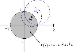
I should immediately add that this domain D will always be an open disk, as illustrated below. The term ‘open’ means that the boundary points (i.e. the circle itself) are not part of the domain. This open disk is the so-called circle of convergence for the complex function f(z) = 1/(1-z), which is equivalent to the (infinite) power series f(z) = 1 + z + z2 + z3 + z4 +… [A clever reader will probably try to check this using Taylor’s theorem above, but I should note the exercise involves some gymnastics. Indeed, the development involves the use of the identity 1 + z + z2 + z3 + … + zn = (1 – zn+1)/(1 – z).]

This power series converges only when the absolute value of z is (strictly) smaller than 1, so only when ¦z¦ < 1. Indeed, the illustration above shows the singularity at the point 1 (or the point (1, 0) if you want) on the real axis: the denominator of the function 1/(1-z) effectively becomes zero there. But so that’s one point only and, hence, we may ask ourselves why this domain should be bounded a circle going through this one point. Why not some square or rectangle or some other weird shape avoiding this point? That question takes a few theorems to answer, and so I’ll just say that this is just one of the many remarkable things about analytic functions: if a power series such as the one above converges to f(z) within some circle whose radius is the distance from z0 (in this case, z0 is the origin and so we’re actually dealing with a so-called Maclaurin expansion here, i.e. an oft-used special case of the Taylor expansion) to the nearest point z1 where f fails to be analytic (that point z1 is equal to 1 in this case), then this circle will actually be the largest circle centered at z0 such that the series converges to f(z) for all z interior to it.
Puff… That’s quite a mouthful so let me rephrase it. What is being said here is that there’s usually a condition of validity for the power series expansion of a function: if that condition of validity is not fulfilled, then the function cannot be represented by the power series. In this particular case, the expansion of f(z) = 1/(1-z) = 1 + z + z2 + z3 + z4 +… is only valid when ¦z¦ < 1, and so there is no larger circle about z0 (i.e. the origin in this particular case) such that at each point interior to it, the Taylor series (or the Maclaurin series in this case) converges to f(z).
That being said, we can usually work our way around such singularities, especially when they are isolated, such as in this example (there is only this one point 1 that is causing trouble), and that is where the concept of analytic continuation comes in. However, before I explain this, I should first introduce Laurent’s theorem, which is like Taylor’s theorem but it applies to functions which are not as ‘nice’ as the functions for which Taylor’s theorem holds (i.e. functions that are not analytic everywhere), such as this 1/(1-z) function indeed. To be more specific, Laurent’s theorem says that, if we have a function f which is analytic in an annular domain (i.e. the red area in the illustration below) centered at some point z0 (in the illustration below, that’s point c) then f(z) will have a series representation involving both positive and negative powers of the term (z – z0).
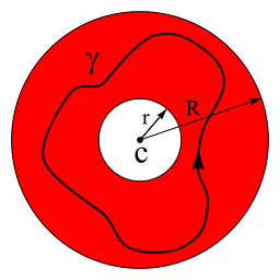
More in particular, f(z) will be equal to f(z) = ∑ [an(z – z0)n] + ∑ [bn/(z-z0)n], with n = 0, 1,…, ∞ and with an and bn coefficients involving complex integrals which I will not write them down here because WordPress lacks a good formula editor and so it would look pretty messy. An alternative representation of the Laurent series is to write f(z) as f(z) = ∑ [cn(z – z0)n], with cn = (1/2πi) ∫C [f(z)/(z – z0)n+1]dz (n = 0, ±1, ±2,…, ±∞). Well – so here I actually did write down the integral. I hope it’s not too messy 🙂 .
It’s relatively easy to verify that this Laurent series becomes the Taylor series if there would be no singularities, i.e. if the domain would cover the whole disk (so if there would be red everywhere, even at the origin point). In that case, the cn coefficient becomes (1/2πi) ∫C [f(z)/(z – z0)-1+1]dz for n = -1 and we can use the fact that, if f(z) is analytic everywhere, the integral ∫C [f(z)dz will be zero along any contour in the domain of f(z). For n = -2, the integrand becomes f(z)/(z – z0)-2+1 = f(z)(z – z0) and that’s an analytic function as well because the function z – z0 is analytic everywhere and, hence, the product of this (analytic) function with f(z) will also be analytic everywhere (sums, products and compositions of analytic functions are also analytic). So the integral will be zero once again. Similarly, for n = -3, the integrand f(z)/(z – z0)-3+1 = f(z)(z – z0)2 is analytic and, hence, the integral is again zero. In short, all bn coefficients (i.e. all ‘negative’ powers) in the Laurent series will be zero, except for n = 0, in which case bn = b0 = a0. As for the an coefficients, one can see they are equal to the Taylor coefficients by using what Penrose refers to as the ‘higher-order’ version of the Cauchy integral formula: f(n)(z0)/n! = (1/2πi) ∫C [f(z)/(z – z0)n+1]dz.
It is also easy to verify that this expression also holds for the special case of a so-called punctured disk, i.e. an annular domain for which the ‘hole’ at the center is limited to the center point only, so this ‘annular domain’ then consists of all points z around z0 for which 0 < ¦z – z0¦ < R. We can then write the Laurent series as f(z) = ∑ an(z-z0)n + b1/(z – z0) + b2/(z – z0)2 +…+ bn/(z – z0)n +… with n = 0, 1, 2,…, ∞.
OK. So what? Well… The point to note is that we can usually deal with singularities. That’s what the so-called theory of residues and poles is for. The term pole is a more illustrious term for what is, in essence, an isolated singular point: it has to do with the shape of the (modulus) surface of f(z) near this point, which is, well… shaped like a tent on a (vertical) pole indeed. As for the term residue, that’s a term used to denote this coefficient b1 in this power series above. The value of the residue at one or more isolated singular points can be used to evaluate integrals (so residues are used for solving integrals), but we won’t go into any more detail here, especially because, despite my initial promise, I still haven’t explained what analytic continuation actually is. Let me do that now.
For once, I must admit that Penrose’s explanation here is easier to follow than other texts (such as the Wikipedia article on analytic continuation, which I looked at but which, for once, seems to be less easy to follow than Penrose’s notes on it), so let me closely follow his line of reasoning here.
If, instead of the origin, we would use a non-zero point z0 for our expansion of this function f(z) = 1/(1-z) = 1 + z + z2 + z3 + z4 +… (i.e. a proper Taylor expansion, instead of the Maclaurin expansion around the origin), then we would, once again, find a circle of convergence for this function which would, once again, be bounded by the singularity at point (1, 0), as illustrated below. In fact, we can move even further out and expand this function around the (non-zero) point z1 and so on and so on. See the illustration: it is essential that the successive circles of convergence around the origin, z0, z1 etcetera overlap when ‘moving out’ like this.
So that’s this concept of ‘analytic continuation’. Paraphrasing Penrose, what’s happening here is that the domain D of the analytic function f(z) is being extended to a larger region D’ in which the function f(z) will also be analytic (or holomorphic – as this is the term which Penrose seems to prefer over ‘analytic’ when it comes to complex-valued functions).
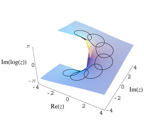
Now, we should note something that, at first sight, seems to be incongruent: as we wander around a singularity like that (or, to use the more mathematically correct term, a pole of the function) to then return to our point of departure, we may get (in fact, we are likely to get) different function values ‘back at base’. Indeed, the illustration below shows what happens when we are ‘wandering’ around the origin for the log z function. You’ll remember (if not, see the previous posts) that, if we write z using polar coordinates (so we write z as z = reiθ), then log z is equal to log z = lnr + i(θ + 2nπ). So we have a multiple-valued function here and we dealt with that by using branches, i.e. we limited the values which the argument of z (arg z = θ) could take to some range α < θ < α + 2π. However, when we are wandering around the origin, we don’t limit the range of θ. In fact, as we are wandering around the origin, we are effectively constructing this Riemann surface (which we introduced in one of our previous posts also), thereby effectively ‘gluing’ successive branches of the log z function together, and adding 2πi to the value of our log z function as we go around. [Note that the vertical axis in the illustration below keeps track of the imaginary part of log z only, i.e. the part with θ in it only. If my imaginary reader would like to see the real part of log z, I should refer him to the post with the entry on Riemann surfaces.]
But what about the power series? Well… The log z function is just like any other analytic function and so we can and do expand it as we go. For example, if we expand the log z function about the point (1, 0), we get log z = (z – 1) – (1/2)(z – 1)2 + (1/3)(z – 1)3 – (1/4)(z – 1)4 +… etcetera. But as we wonder around, we’ll move into a different branch of the log z function and, hence, we’ll get a different value when we get back to that point. However, I will leave the details of figuring that one out to you 🙂 and end this post, because the intention here is just to illustrate the principle, and not to copy some chapter out of a math course (or, at least, not to copy all of it let’s say :-)).
If you can’t work out it out, you can always try to read the Wikipedia article on analytic continuation. While less ‘intuitive’ than Penrose’s notes on it, it’s definitely more complete, even if does not quite exhaust the topic. Wikipedia defines analytic continuation as “a technique to extend the domain of a given analytic function by defining further values of that function, for example in a new region where an infinite series representation in terms of which it is initially defined becomes divergent.” The Wikipedia article also notes that, “in practice, this continuation is often done by first establishing some functional equation on the small domain and then using this equation to extend the domain: examples are the Riemann zeta function and the gamma function.” But so that’s sturdier stuff which Penrose does not touch upon – for now at least, but I expect him to develop such things in later Road to Reality chapters).
Post scriptum: Perhaps this is an appropriate place to note that, at first sight, singularities may look like no big deal: so we have a infinitesimally small hole in the domain of function log z or 1/z s or whatever, so what? Well… It’s probably useful to note that, if we wouldn’t have that ‘hole’ (i.e. the singulariy), any integral of this function (I mean the integral of this function along any closed contour around that point, i.e. ∫C f(z)dz, would be equal to zero, but when we do have that little hole, like for f(z) = 1/z, we don’t have that result. In this particular case (i.e. f(z) = 1/z), you should note that the integral ∫C (1/z)dz, for any closed contour around the origin, equals 2πi, or that, just to give one more example here, that the value of the integral ∫C [f(z)/(z – z0)]dz is equal to 2πi f(z0). Hence, even if f(z) would be analytic over the whole open disk, including the origin, the ‘quotient function’ f(z)/z will not be analytic at the origin and, hence, the value of the integral of this ‘quotient function’ f(z)/z around the origin will not be zero but equal to 2πi times the value of the original f(z) function at the origin, i.e. 2πi times f(0). Vice versa, if we find that the value of the integral of some function around a closed contour – and I mean any closed contour really – is not equal to zero, we know we’ve got a problem somewhere and so we should look out for one or more infinitesimally small little ‘holes’ somewhere in the domain. Hence, singularities, and this complex theory of poles and residues which shows us how we can work with them, is extremely relevant indeed: it’s surely not a matter of just trying to get some better approximation for this or that value or formula or so. 🙂
In light of the above, it is now also clear that the term ‘residue’ is well chosen: this coefficient b1 is equal to ∫C f(z)dz divided by 2πi (I take the case of a Maclaurin expansion here) and, hence, there would be no singularity, this integral (and, hence, the coefficient b1) would be equal to zero. Now, because of the singularity, we have a coefficient b1 ≠ 0 and, hence, using the term ‘residue’ for this ‘remnant’ is quite appropriate.
