
Pre-scriptum (dated 26 June 2020): In pre-scriptums for my previous posts on math, I wrote that the material in posts like this remains interesting but that one, strictly speaking, does not need it to understand quantum mechanics. This post is a little bit different: one has to understand the basic concept of a differential equation as well as the basic solution methods. So, yes, it is a prerequisite. ![]()
Original post:
Although Richard Feynman’s iconic Lectures on Physics are best read together, as an integrated textbook that is, smart publishers bundled some of the lectures in two separate publications: Six Easy Pieces and Six Not-So-Easy Pieces. Well… Reading Penrose has been quite exhausting so far and, hence, I feel like doing an easy piece here – just for a change. 🙂
In addition, I am half-way through this graduate-level course on Complex variables and Applications (from McGraw-Hill’s Brown—Churchill Series) but I feel that I will gain much more from the remaining chapters (which are focused on applications) if I’d just branch off for a while and first go through another classic graduate-level course dealing with math, but perhaps with some more emphasis on physics. A quick check reveals that Mathematical Methods of Physics, written by Jon Mathews and R.L. Walker will probably fit the bill. This textbook is used it as a graduate course at the University of Chicago and, in addition, Mathews and Walker were colleagues of Feynman and, hence, their course should dovetail nicely with Feynman’s Lectures: that’s why I bought it when I saw this 2004 reprint for the Indian subcontinent in a bookshop in Delhi. [As for Feynman’s Lectures, I wouldn’t recommend these Lectures if you want to know more about quantum mechanics, but for classical mechanics and electromagnetism/electrodynamics they’re still great.]
So here we go: Chapter 1, on Differential Equations.
Of course, I mean ordinary differential equations, so things with one dependent and one independent variable only, as opposed to partial differential equations, which have partial derivatives (i.e. terms with δ symbols in them, as opposed to the d used in dy and dy) because there’s more than one independent variable. We’ll need to get into partial differential equations soon enough, if only because wave equations are partial differential equations, but let’s start with the start.
While I thought I knew a thing or two about differential equations from my graduate-level courses in economics, I’ve discovered many new things already. One of them is the concept of a slope field, or a direction field. Below the examples I took from Paul’s Online Notes in Mathematics (http://tutorial.math.lamar.edu/Classes/DE/DirectionFields.aspx), who’s a source I warmly recommend (his full name is Paul Dawkins, and he developed these notes for Lamar University, Texas):
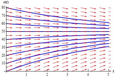
These things are great: they helped me to understand what a differential equation actually is. So what is it then? Well, let’s take the example of the first graph. That example models the following situation: we have a falling object with mass m (so the force of gravity acts on it) but its fall gets slowed down because of air resistance. So we have two forces FG and FA acting on the object, as depicted below:
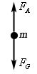
Now, the force of gravity is proportional to the mass m of the falling object, with the factor of proportionality equal to the gravitational constant of course. So we have FG = mg with g = 9.8 m/s2. [Note that forces are measured in newtons and 1 N = 1 (kg)(m)/(s2).]
The force due to air resistance has a negative sign because it acts like a brake and, hence, it has the opposite direction of the gravity force. The example assumes that it is proportional to the velocity v of the object, which seems reasonable enough: if it goes faster and faster, the air will slow it down more and more so we have FA = —γv, with v = v(t) the velocity of the object and γ some (positive) constant representing the factor of proportionality for this force. [In fact, the force due to air resistance is usually referred to as the drag, and it is proportional to the square of the velocity, but so let’s keep it simple here.]
Now, when things are being modeled like this, I find the thing that is most difficult is to keep track of what depends on what exactly. For example, it is obvious that, in this example, the total force on the object will also depend on the velocity and so we have a force here which we should write as a function of both time and velocity. Newton’s Law of Motion (the Second Law to be precise, i.e. ma = m(dv/dt) =F) thus becomes
m(dv/dt) = F(t, v) = mg – γv(t).
Note the peculiarity of this F(t, v) function: in the end, we will want to write v(t) as an explicit function of t, but so here we write F as a function with two separate arguments t and v. So what depends on what here? What does this equation represent really?
Well… The equation does surely not represent one or the other implicit function: an implicit function, such as x2 + y2 = 1 for example (i.e. the unit circle), is still a function: it associates one of the variables (usually referred to as the value) to the other variables (the arguments). But, surely, we have that too here? No. If anything, a differential equation represents a family of functions, just like an indefinite integral.
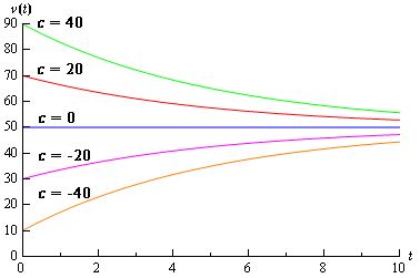
Indeed, you’ll remember that an indefinite integral ∫f(x)dx represents all functions F(x) for which F'(x) = dF(x)/dx = f(x). These functions are, for a very obvious reason, referred to as the anti-derivatives of f(x) and it turns out that all these antiderivatives differ from each other by a constant only, so we can write ∫f(x)dx = F(x) + c, and so the graphs of all the antiderivatives of a given function are, quite simply, vertical translations of each other, i.e. their vertical location depends on the value of c. I don’t want to anticipate too much, but so we’ll have something similar here, except that our ‘constant’ will usually appear in a somewhat more complicated format such as, in this example, as v(t) = 50 + ce—0.196t. So we also have a family of primitive functions v(t) here, which differ from each other by the constant c (and, hence, are ‘indefinite’ so to say), but so when we would graph this particular family of functions, their vertical distance will not only depend on c but also on t. But let us not run before we can walk.
The thing to note – and to always remember when you’re looking at a differential equation – is that the equation itself represents a world of possibilities, or parallel universes if you want :-), but, also, that’s it in only one of them that things are actually happening. That’s why differential equations usually have an infinite number of general (or possible) solutions but only one of these will be the actual solution, and which one that is will depend on the initial conditions, i.e. where we actually start from: is the object at rest when we start looking, is it in equilibrium, or is it somewhere in-between?
What we know for sure is that, at any one point of time t, this object can only have one velocity, and, because it’s also pretty obvious that, in the real world, t is the independent variable and v the dependent one (the velocity of our object does not change time), we can thus write v = v(t) = du/dt indeed. [The variable u = u(t) is the vertical position of the object and its velocity is, obviously, the rate of change of this vertical position, i.e. the derivative with regard to time.]
So that’s the first thing you should note about these direction fields: we’re trying to understand what is going on with these graphs and so we identify the dependent variable with the y axis and the independent variable with the x axis, in line with the general convention that such graphs will usually depict a y = y(x) relationship. In this case, we’re interested in the velocity of the object (not its position), and so v = v(t) is the variable on the y axis of that first graph.
Now, there’s a world of possibilities out there indeed, but let’s suppose we start watching when the object is at rest, i.e. we have v(t) = v(0) = 0 and so that’s depicted by the origin point. Let’s also make it all more real by assigning the values m = 2 kg and γ = 0.392 to m an γ in Newton’s formula. [In case you wonder where this value for γ comes from, note that its value is 1/25 of the gravitational constant and so it’s just a number to make sure the solution for v(t) is a ‘nice’ number, i.e. an integer instead of some decimal. In any case, I am taking this example from Paul’s Online Notes and I won’t try to change it.]
So we start at point zero with zero velocity but so now we’ve got the force F with us. 🙂 Hence, the object’s velocity v(t) will not stay zero. As the clock ticks, its movement will respect Newton’s Law, i.e. m(dv/dt) = F(t, v), which is m(dv/dt) = mg – γv(t) in this case. Now, if we plug in the above-mentioned values for m and γ (as well as the 9.8 approximation for g), we get dv(t)/dt = 9.8 – 0.196v(t) (we brought m over to the other side, and so then it becomes 1/m on the right-hand side).
Now, let’s insert some values into these equation. Let’s first take the value v(0) = 0, i.e. our point of departure. We obviously get d(v(0)/dt = 9.8 – 0.196.0 = 9.8 (so that’s close to 10 but not quite).
Let’s take another value for v(0). If v(0) would be equal to 30 m/s (this means that the object is already moving at a speed of 30 m/s when we start watching), then we’d get a value for dv/dt of 3.92, which is much less – but so that reflects the fact that, at such speed, air resistance is counteracting gravity.
Let’s take yet another value for v(0). Let’s take 100 now for example: we get dv/dt = – 9.8.
Ooops! What’s that? Minus 9.8? A negative value for dv/dt? Yes. It indicates that, at such high speed, air resistance is actually slowing down the object. [Of course, if that’s the case, then you may wonder how it got to go so fast in the first place but so that’s none of our own business: maybe it’s an object that got launched up into the air instead of something that was dropped out of an airplane. Note that a speed of 100 m/s is 360 km/h so we’re not talking any supersonic launch speeds here.]
OK. Enough of that kids’ stuff now. What’s the point?
Well, it’s these values for dv/dt (so these values of 9.8, 3.92, -9.8 etcetera) that we use for that direction field, or slope field as it’s often referred to. Note that we’re currently considering the world of possibilities, not the actual world so to say, and so we are contemplating any possible combination of v and t really.
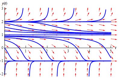
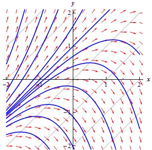
Also note that, in this particular example that is, it’s only the value of v that determines the value of dv/dt, not the value of t. So, if, at some other point in time (e.g. t = 3), we’d be imagining the same velocities for our object, i.e. 0 m/s, 30 m/s or 100 m/s, we’d get the same values 9.8, 3.92 and -9.8 for dv/dt. So the little red arrows which represent the direction field all have the same magnitude and the same direction for equal values of v(t). [That’s also the case in the second graph above, but not for the third graph, which presents a far more general case: think of a changing electromagnetic field for instance. A second footnote to be made here concerns the length – or magnitude – of these arrows: they obviously depend on the scale we’re using but so they do reflect the values for dv/dt we calculated.]
So that slope field, or direction field, i.e. all of these little red arrows, represents the fact that the world of possibilities, or all parallel universes which may exist out there, have one thing in common: they all need to respect Newton or, at the very least, his m(dv/dt) = mg – γv(t) equation which, in this case, is dv(t)/dt = 9.8 – 0.196v(t). So, wherever we are in this (v, t) space, we look at the nearest arrow and it will tell us how our speed v will change as a function of t.
As you can see from the graph, the slope of these little arrows (i.e. dv/dt) is negative above the v(t) = 50 m/s line, and positive underneath it, and so we should not be surprised that, when we try to calculate at what speed dv/dt would be equal to zero (we do this by writing 9.8 – 0.196v(t) = 0), we find that this is the case if and only if v(t) = 9.8/0.196 = 50 indeed. So that looks like the stable situation: indeed, you’ll remember that derivatives reflect the rate of change, and so when dv/dt = 0, it means the object won’t change speed.
Now, the dynamics behind the graph are obviously clear: above the v(t) = 50 m/s line, the object will be slowing down, and underneath it, it will be speeding up. At the v(t) line itself, the gravity and air resistance forces will balance each other and the object’s speed will be constant – that is until it hits the earth of course :-).
So now we can have a look at these blue lines on the graph. If you understood something of the lengthy story about the red arrows above, then you’ll also understand, intuitively at least, that the blue lines on this graph represent the various solutions to the differential equation. Huh? Well. Yes.
The blue lines show how the velocity of the object will gradually converge to 50 m/s, and that the actual path being followed will depend on our actual starting point, which may be zero, less than 50 m/s, or equal or more than 50 m/s. So these blue lines still represent the world of possibilities, or all of the possible parallel universes, but so one of them – and one of them only – will represent the actual situation. Whatever that actual situation is (i.e. whatever point we start at when t = 0), the dynamics at work will make sure the speed converges to 50 m/s, so that’s the longer-term equilibrium for this situation. [Note that all is relative of course: if the object is being dropped out of a plane at an altitude of two or three km only, then ‘longer-term’ means like a minute or so, after which time the object will hit the ground and so then the equilibrium speed is obviously zero. :-)]
OK. I must assume you’re fine with the intuitive interpretation of these blue curves now. But so what are they really, beyond this ‘intuitive’ interpretation? Well, they are the solutions to the differential equation really and, because these solutions are found through an integration process indeed, they are referred to as the integral curves. I have to refer my imaginary reader here to Paul’s Notes (or any other math course) for as to how exactly that integration process works (it’s not as easy as you might think) but the equation for these blue curves is
v(t) = 50 + ce—0.196t
In this equation, we have Euler’s number e (so that’s the irrational number e = 2.718281… etcetera) and also a constant c which depends on the initial conditions indeed. The graph below shows some of these curves for various values of c. You can calculate some more yourself of course. For example, if we start at the origin indeed, so if we have zero speed at t = 0, then we have v(0) = 50 + ce-0.196.0 = 50 + ce0 = 50 + c and, hence, c = -50 will represent that initial condition. [And, yes, please do note the similarity with the graphs of the antiderivatives (i.e. the indefinite integral) of a given function, because the c in that v(t) function is, effectively, the result of an integration process.]
So that’s it really: the secret behind differential equations has been unlocked. There’s nothing more to it.
Well… OK. Of course we still need to learn how to actually solve these differential equations, and we’ll also have to learn how to solve partial differential equations, including equations with complex numbers as well obviously, and so on and son on. Even those other two ‘simple’ situations depicted above (see the two other graphs) are obviously more intimidating already (the second graph involves three equilibrium solutions – one stable, one unstable and one semi-stable – while the third graph shows not all situations have equilibrium solutions). However, I am sure I’ll get through it: it has been great fun so far, and what I read so far (i.e. this morning) is surely much easier to digest than all the things I wrote about in my other posts. 🙂
In addition, the example did involve two forces, and so it resembles classical electrodynamics, in which we also have two forces, the electric and magnetic force, which generate force fields that influence each other. However, despite of all the complexities, it is fair to say that, when push comes to shove, understanding Maxwell’s equations is a matter of understanding a particular set of partial differential equations. However, I won’t dwell on that now. My next post might consist of a brief refresher on all of that but I will probably first want to move on a bit with that course of Mathews and Walker. I’ll keep you posted on progress. 🙂
Post scriptum:
My imaginary reader will obviously note that this direction field looks very much like a vector field. In fact, it obviously is a vector field. Remember that a vector field assigns a vector to each point, and so a vector field in the plane is visualized as a collection of arrows indeed, with a given magnitude and direction attached to a point in the plane. As Wikipedia puts it: ‘vector fields are often used to model the strength and direction of some force, such as the electrostatic, magnetic or gravitational force. And so, yes, in the example above, we’re indeed modeling a force obeying Newton’s law: the change in the velocity of the object (i.e. the factor a = dv/dt in the F = ma equation) is proportional to the force (which is a force combining gravity and drag in this example), and the factor of proportionality is the inverse of the object’s mass (a = F/m and, hence, the greater its mass, the less a body accelerates under given force). [Note that the latter remark just underscores the fact that Newton’s formula shows that mass is nothing but a measure of the object’s inertia, i.e. its resistance to being accelerated or change its direction of motion.]
A second post scriptum point to be made, perhaps, is my remark that solving that dv(t)/dt = 9.8 – 0.196v(t) equation is not as easy as it may look. Let me qualify that remark: it actually is an easy differential equation, but don’t make the mistake of just putting an integral sign in front and writing something like ∫(0.196v + v’) dv = ∫9.8 dv, to then solve it as 0.098 v2 + v = 9.8v + c, which is equivalent to 0.098 v2 – 8.8 v + c = 0. That’s nonsensical because it does not give you v as an implicit or explicit function of t and so it’s a useless approach: it just yields a quadratic function in v which may or may not have any physical interpretation.
So should we, perhaps, use t as the variable of integration on one side and, hence, write something like ∫(0.196v + v’) dv = ∫9.8 dt? We then find 0.098 v2 + v = 9.8t + c, and so that looks good, doesn’t it? No. It doesn’t. That’s worse than that other quadratic expression in v (I mean the one which didn’t have t in it), and a lot worse, because it’s not only meaningless but wrong – very wrong. Why? Well, you’re using a different variable of integration (v versus t) on both sides of the equation and you can’t do that: you have to apply the same operation to both sides of the equation, whether that’s multiplying it with some factor or bringing one of the terms over to the other side (which actually mounts to subtracting the same term from both sides) or integrating both sides: we have to integrate both sides over the same variable indeed.
But – hey! – you may remember that’s what we do when differential equations are separable, isn’t? And so that’s the case here, isn’t it?We’ve got all the y’s on one side and all the x’s on the other side of the equation here, don’t we? And so then we surely can integrate one side over y and the other over x, isn’t it? Well… No. And yes. For a differential equation to be separable, all the x‘s and all the y’s must be nicely separated on both sides of the equation indeed but all the y’s in the differential equation (so not just one of them) must be part of the product with the derivative. Remember, a separable equation is an equation in the form of B(y)(dy/dx) = A(x), with B(y) some function of y indeed, and A(x) some function of x, but so the whole B(y) function is multiplied with dy/dx, not just one part of it. If, and only if, the equation can be written in this form, we can (a) integrate both sides over x but (b) also use the fact that ∫[B(y)dy/dx]dx = ∫B(y)dy. So, it looks like we’re effectively integrating one part (or one side) of the equation over the dependent variable y here, and the other over x, but the condition for being allowed to do so is that the whole B(y) function can be written as a factor in a product involving the dy/dx derivative. Is that clear? I guess not. 😦 But then I need to move on.
The lesson here is that we always have to make sure that we write the differential equation in its ‘proper form’ before we do the integration, and we should note that the ‘proper form’ usually depends on the method we’re going to select to solve the equation: if we can’t write the equation in its proper form, then we can’t apply the method. […] Oh… […] But so how do we solve that equation then? Well… It’s done using a so-called integrating factor but, just as I did in the text above already, I’ll refer you to a standard course on that, such as Paul’s Notes indeed, because otherwise my posts would become even longer than they already are, and I would have even less imaginary readers. 🙂
