
This post has got nothing to do with quantum mechanics. It’s just… Well… My son – who’s preparing for his entrance examinations for engineering studies – sent me a message yesterday asking me to quickly explain Davidson’s function – as he has to do some presentation on it as part of a class assignment. As I am an economist – and Davidson’s function is used in transport economics – he thought I would be able to help him out quickly, and I was. So I just thought it might be interesting to quickly jot down my explanation as a post in this blog. It won’t help you with quantum mechanics but, if anything, it may help you think about functional forms and some related topics.
In his message, he sent me the function – copied below – and some definitions of the variables which he got from some software package he had seen or used – at least that’s what he told me. 🙂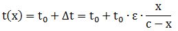 So… This function tells us that the dependent variable is the travel time t, and that it is seen as a function of some independent variable x and some parameters t0, c and ε. My son defined the variable x as the flow (of vehicles) on the road, and c as the capacity of the road. To be precise, he wrote the formula that was to be used for c as follows:
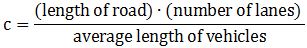 What about a formula for x? Well… He said that was the actual flow of vehicles, but he had no formula for it. As for t0, that was the travel time “at free speed.” Finally, he said ε was a “paramètre de sensibilité de congestion.” Sorry for the French, but that’s the language of his school, which is located in some town in southern Belgium. In English, we might translate it as a congestion sensitivity coefficient. And so that’s what he struggled most with – or so he said.
So that got us started. I immediately told him that, if you write something like c − x, then you’d better make sure c and x have the same physical dimension. The formula above tells us that c is the number of vehicles that you can park on that road. Bumper to bumper. So I told him that’s a rather weird definition of capacity. It’s definitely not the dimension of flow: the flow should be some number per second or – much more likely in transport economics – per minute or per hour. So I told him that he should double-check those definitions of x and c, and that I’d get back to him to explain the formula itself after I had googled and read some articles on it. So I did that, and so here’s the full explanation I gave him.
While there’s some pretty awesome theory behind (queuing theory and all that), which transportation gurus take very seriously – see, for example, the papers written by Rahmi Akçelik – a quick look at it all reveals that Davidson’s function is, essentially, just a specific functional form that we impose on some real-life problem. So I’d call it an empirical function: there’s some theory behind, but it’s more based on experience than pure theory. Of course, sound logic is – or should be – applied to both empirical as well as to purely theoretical functions, but… Well… It’s a different approach than, say, modeling the dynamics of quantum-mechanical state changes. 🙂 Just note, for example, that we might just as well have tried something else – some exponential function. Something like this, for example: Davidson’s function is, quite simply, just nicer and easier than the one above, because the function above is not linear. It could be quadratic (β = 2), or whatever, but surely not linear. In contrast, Davidson’s function is linear and, therefore, easy to fit onto actual traffic data using the simplest of simple linear regression models – and, speaking from experience, most engineers and economists in a real-life job can barely handle even that! 🙂
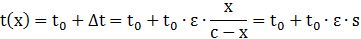
So just look at that x/(c−x) factor as measuring the congestion or saturation, somehow. We’ll denote it by s. If you can sort of accept that, then you’ll agree that Davidson’s function tells us that the extra time that’s needed to drive from some place a to some place b along our road will be directly proportional to:
- That congestion factor x/(c−x), about which I’ll write more in a moment;
- The free-speed or free-flow travel time t0 – which I’ll call the free-flow travel time from now on, rather than the free-speed travel time, because there’s no such thing as free speed in reality: we have speed limits – or safety limits, or scared moms in the car, whatever – and, a more authoritative argument, the literature on Davidson’s function also talks about free flow rather than free speed;
- That epsilon factor (ε), which – of all the stuff I presented so far – mystified my son most.
So the formula for the extra travel time that’s needed is, obviously, equal to: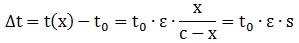 So we have a very simple linear functional form for the extra travel time, and we can easily estimate the actual value of our ε parameter using actual traffic data in a simple linear regression. The data analysis toolkit of MS Excel will do stuff like this – if you have the data, of course – so you don’t need a sophisticated statistical software package here.
So that’s it, really: Davidson’s function is, effectively, just nice and easy to work with. […] Well… […] Of course, we still need to define what x and c actually are. And what’s that so-called free flow (or free speed?) travel time? Well… The free-flow travel time is, obviously, the time you need to go from a to b at the free-flow speed. But what’s the free-flow speed? My friend’s Maserati is faster than my little Santro. 🙂 And are we allowed to go faster than the maximum authorized speed? Interesting questions.
So that’s where the analysis becomes interesting, and why we need better definitions of x and c. If c is some density – what my son’s rather non-sensical formula seems to imply – we may want to express it per unit distance. Per kilometer, for example. So we should probably re-define c more simply: as the number of lanes divided by the average length of the vehicles that are using it. We get that by dividing the c above by the length of the road – so we divide the length of the road by the length of the road, which gives 1. 🙂 You may think that’s weird, because we get something like 3/5 = 0.6… So… What? Well… Yes. 0.6 vehicles per meter, so that’s 600 vehicles per kilometer! Does that sound OK? I think it does. So let’s express that capacity (c) as a maximum density – for the time being, at least.
Now, none of those cars can move, of course: they are all standing still. Bumper to bumper. It’s only when we decrease the density that they’re able to move. In fact, you can – and should – visualize the process: the first car moves and opens a space of, say, one or two meter, and then the second one, and so and so on – till all cars are moving with a few meter in-between them. So the density will obviously decrease and, as a result, we’re getting some flow of vehicles here. If there’s three meter between them, for example, then the density goes down to 3/8 vehicles per meter, so that’s 375 vehicles per kilometer. Still a lot, and you’ll have to agree that – with only 3 meters between them – they’ll probably only move very slowly!
You get the idea. We can now define x as a density too – some density x that is smaller than the maximum density c. Then that x/(c−x) factor – measuring the saturation – obviously makes a lot of sense. The graph below shows how it looks like for c = 5. [The value of 5 is just random, and its order of magnitude doesn’t matter either: we can always re-scale from m to km, or from seconds to minutes and what have you. So don’t worry about it.] Look at this example: when x is small – like 1 or 2 only – then x/(5−x) doesn’t increase all that much. So that means we add little to the travel time. Conversely, when x approaches c = 5 – so that’s the limit (as you can see, the x = 5 line is a (vertical) asymptote of the function) – then the travel time becomes huge and starts approaching infinity. So… Well… Yes. That’s when all cars are standing still – bumper to bumper.  But so what’s the free-flow speed? Is it the maximum speed of my friend’s Maserati -which is like 275 km/h? Well… I don’t think my friend ever drove that fast, so probably not. What else? Think about it. What should we choose here? The obvious choice is the speed limit: 120 km/h, or 90 km/h, or 60 km/h – or whatever. Why? Because you don’t want a ticket, I guess… In any case, let’s analyze that question later. Let’s first look at something else.
Of course, you’ll want to keep some distance between you and the car in front of you when driving at relatively high speeds, and that’s the crux of the analysis really. You may or, more likely, you may not remember that your driving instructor told you to always measure the safety distance between you and the car(s) in front in seconds rather than in meter. In Belgium, we’re told to stay two seconds away from the car in front of us. So when it passes a light pole, we’ll count “twenty-one, twenty-two” and… Well… If we pass that same light pole while we’re still counting those two seconds, then we’d better keep some more distance. It’s got to do with reaction time: when the car in front of you slams the brakes, you need some time to react, and then that car might also have better brakes than yours, so you want to build in some extra safety margin in case you don’t slow down as fast as the car in front of you. So that two-seconds rule is not about the breaking distance really – or not about the breaking distance alone. No. It’s more about the reaction time. In any case, the point is that you’ll want to measure the safety distance in time rather than in meter. Capito? OK… Onwards…
Now, 120 km/h amounts to 120,000/3,600 = 33.333 meter per second. So the safety distance here is almost 67 meter! If the maximum authorized velocity is only 90 km/h, then the safety distance shrinks to 2 × (90,000/3,600) = 50 meter. For a maximum authorized velocity of 60 km/h, the safety distance would be equal to 33.333 meter. Both are much larger distances than the average length of the vehicles and, hence, it’s basically the safety distance – not the length of the vehicle – that we need to consider! Let’s quickly calculate the related densities:
- For a three-lane highway, with all vehicles traveling at 120 km/h and keeping their safety distance, the density will be equal to 3·1,000/66.666… = 45 vehicles per kilometer of highway, so that’s 15 vehicles per lane.
- If the travel speed is 90 km/h, then the density will be equal to 60 vehicles per km (20 vehicles per lane).
- Finally, at 60 km/h, the density will be 90 vehicles per km (30 vehicles per lane).
Note that our two-seconds rule implies a linear relation between the safety distance and the maximum authorized speed. You can also see that the relation between the density and the maximum authorized speed is inversely proportional: if we halve the speed, the density doubles.
Now, you can easily come up with some more formulas, and play around a bit. For example, if we denote the security distance by d, and the mentioned two seconds as td – so that’s the time (t) that defines the security distance d – then d is, logically, equal to: d = td∙vmax. But rather than trying to find more formulas and play with them, let’s think about that concept of flow now. If we would want to define the capacity – or the actual flow – in terms of the number of vehicles that are passing along any point along this highway, how should we calculate that?
Well… The flow is the number of vehicles that will pass us in one hour, right? So if vmax is 120 km/h, then – assuming full capacity – all the vehicles on the next 120 km of highway will all pass us, right? So that makes 45 vehicles per km times 120 km = 5,400 vehicles – per hour, of course. Hence, the flow is just the product of the density times the speed.
Now, look at this: if vmax is equal to 90 km/h, then we’ll have 60 vehicles per km times 90 km = … Well… It’s – interestingly enough – the same number: 5,400 vehicles per hour. Let’s calculate for vmax = 60 km/h… Security distance is 33.333 meter, so we can have 90 vehicles on each km of highway which means that, over one hour, 90 times 60 = 5,400 vehicles will pass us! It’s, once again, the same number: 5,400! Now that’s a very interesting conclusion. Let me highlight it:
If we assume the vehicles will keep some fixed time distance between them (e.g. two seconds), then the capacity of our highway – expressed as some number of vehicles passing along it per time unit – does not depend on the velocity.
So the capacity – expressed as a flow rather than as a density – is just a fixed number: x vehicles per hour. The density affects only the (average) speed of all those vehicles. Hence, increasing densities are associated with lower speeds, and higher travel times, but they don’t change the capacity.
It’s really a rather remarkable conclusion, even if the relation between the density and the flow is easily understood – both mathematically and, more importantly, intuitively. For example, if the density goes down to 60 vehicles per km of highway, then they will only be able to move at a speed of 90 km/h, but we’ll still have that flow of 5,400 vehicles per hour – which we can look at as the capacity but expressed as some flow rather than as a density. Lower densities allow for even higher speeds: we calculated above that a density of 45 vehicles per km would allow them to drive at a maximum speed of 120 km/h, so travel time would be reduced even more, but we’d still have 5,400 vehicles per hour! So… Well… Yes. It all makes sense.
Now what happens if the density is even lower, so we could – theoretically – drive safely, or not so safely, at some speed that’s way above the speed limit? If we have enough cars – say 30 vehicles per km, but all driving more than 120 km/h, while respecting the two-seconds rule – we’d still have the same flow: 5,400 vehicles per hour. And travel time would go down. But so we can think of lower densities and higher speeds but, again, there’s got to be some limit here – a speed limit, safety considerations, a limit to what our engine or our car can do, and, finally, there’s the speed of light too. 🙂 I am just joking, of course, but I hope you see the point. At some point, it doesn’t matter whether or not the density goes down even further: the travel time should hit some minimum. And it’s that minimum – the lowest possible travel time – that you’d probably like to define as t0.
As mentioned, the minimum travel time is associated with some maximum speed, and – after some consideration of the possible candidates for the maximum speed – you’ll agree the speed limit is a better candidate than the 275 km/h limit of my friends’ Maserati Quattroporte. Likewise, you would probably also like to define x0 as the (maximum) density at the speed limit.
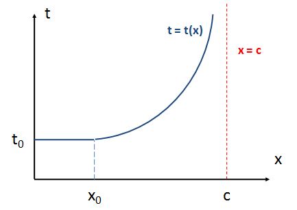
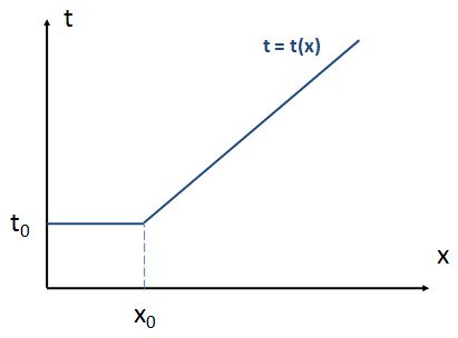
What we’re saying here is that – in theory at least – our t = t(x) function should start with a linear section, between x = 0 and x = x0. That linear section defines a density 0 < x < x0 which is compatible with us driving at the speed limit – say, 120 km/h – and, hence, with us only needing the time t = t0 to arrive at our destination. Only when x becomes larger than x0, we’ve got to reduce speed – below the speed limit (say, 120 km/h) – to keep the flow going while keeping an appropriate safety distance. A reduction of speed implies a increase in travel time, of course. So that’s what’s illustrated in the graph below.
 To be specific, if the speed limit is 120 km/h, then – assuming you don’t want to be caught speeding – the minimum travel time will always be equal to 30 seconds per km, even if you’re alone on the highway. Now, as long as the density is less than 45 vehicles per km, you can keep that travel time the same, because you can do your 120 km/h while keeping the safety distance. But if the density increases, above 45 vehicles per km, then stuff starts slowing down because everyone is uncomfortable with the shorter distance between them and the car in front. As the density goes up even more – say, to 60 vehicles per km – we can only do 90 km/h, and so the travel time will then be equal to 40 seconds per km. And then it goes to 90 vehicles per km, so speed slows down to 60 km/h, and so that’s a travel time of 60 seconds per km. Of course, you’re smart – very smart – and so you’ll immediately say this implies that the second section of our graph should be linear too, like this:
 You’re right. But then… Well… That doesn’t work with our limit for x, which is c. As I pointed out, c is an absolute maximum density: you just can’t park any more cars on that highway – unless you fold them up or so. 🙂 So what’s the conclusion? Well… We may think of the Davidson function as a primitive combination of both shapes, as shown below.
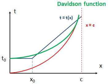
I call it a primitive approximation, because that Davidson function (so that’s the green smooth curve above) is not a precise (linear or non-linear) combination of the two functions we presented (I am talking about the blue broken line and the smooth red curve here). It’s just… Well… Some primitive approximation. 🙂 Now you can write some very complicated papers – as other authors do – to sort of try to explain this shape, but you’ll find yourself fiddling with variable time distance rules and other hypotheses that may or may not make sense. In short, you’re likely to introduce other logical inconsistencies when trying to refine the model. So my advice is to just accept the Davidson’s function as some easy empirical fit to some real-life situation, and think of what the parameters actually do – mathematically speaking, that is. How do they change the shape of our graph?
So we’re now ready to explain that epsilon factor (ε) by looking at what it does, indeed. Please try an online graphing tool with a slider (e.g. https://www.desmos.com/calculator) – just type something like a + bx in the function box, and you’ll see the sliders appear – so you can see how the function changes for different parameter values. The two graphs below, for example, which I made using that graphing tool, show you the function t = 2 + 2∙ε∙x/(10−x) for ε = 0.5 and ε = 10 respectively. As you can see, both functions start at t = 2 and have the same asymptote at x = c = 10. However, you’ll agree that they look very different – and that’s because of the value of the ε parameter. For ε = 0.5, the travel time does not increase all that much – initially at least. Indeed, as you can see, t is equal to 3 if the density is half of the capacity (t = 3 for x = 5 = c/2). In contrast, for ε = 10, we have immediate saturation, so to speak: travel time goes through the roof almost immediately! For example, for x = 3, t ≈ 10.6, so while the density is less than a third of the capacity, the associated travel time is already more than five times the free-flow travel time!


Now I have a tricky question for you: does it make sense to allow ε to take on values larger than one? Think about it. 🙂 In any case, now you’ve seen what the ε factor does from a math point of view. So… Well… I’ll conclude here by just noting that it does, indeed, make sense to refer to ε as a “paramètre de sensibilité de congestion”, because that’s what it is: a congestion sensitivity coefficient. Indeed, it’s not the congestion or saturation parameter itself (that’s a term we should reserve term for the x/(c–x) factor), but a congestion sensitivity coefficient alright!
Of course, you will still want some theoretical interpretation. Well… To be honest, I can’t give you one. I don’t want to get lost in all of those theoretical excursions on Davidson’s function, because… Well… It’s no use. That ε is just what it is: it’s a proportionality coefficient that we are imposing upon our functional form for our travel-time function. You can sum it up as follows:
If x/(c−x) is the congestion parameter (or variable, I should say), then it goes from 0 to ∞ (infinity) when the traffic flow (x) goes x = 0 to x = c (full capacity). So, yes, we can call the x/(c−x) factor the congestion or saturation variable and write it as s = x/(c−x). And then we can refer to ε as the “paramètre de sensibilité de congestion”, because it is a measure not of the congestion itself, but of the sensitivity of the travel time to the congestion.
If you’d absolutely want some mathematical formula for it, then you could use this one, which you get from re-writing Δt = t0·ε·s as Δt/t0 = ε·s:
∂(Δt/t0)/∂s = ε
But… Frankly. You can stare at this formula for a long while – it’s a derivative alright, and you know what derivatives stand for – but you’ll probably learn nothing much from it. [Of course, please write me if you don’t agree, Vincent!] I just looked at those two graphs, and note how their form changes as a function of ε. Perhaps you have some brighter idea about it!
So… Well… I am done. You should now fully understand Davidson’s function. Let me write it down once more:
Again, as mentioned, its main advantage is its linearity. Because of its linearity, it is easy to actually estimate the parameters: it’s just a simple linear regression – using actual travel times and actual congestion measurements – and so then we can estimate the value of ε and see if it works. Huh? How do we see if it works? Well… I told you already: when everything is said and done, Davidson’s function is just one of the many models for the actual reality, so it tries to explain how travel time increases because of congestion. There are other models, which come with other functions – but they are more complicated, and so are the functions that come with them (check out that paper from Rahmi Akçelik, for example). Only reality can tell us what model is the best fit to whatever it is that we’re trying to model. So that’s why I call Davidson’s function an empirical function, and so you should check it against reality. That’s when a statistical software package might be handy: it allows you to test the fit of various functional – linear and non-linear – forms against a real-life data set.
So that’s it. I tasked my son to go through this post and correct any errors – only typos, I hope! – I may have made. I hope he’ll enjoy this little exercise. 🙂
