Comments on the MIT’s Stern-Gerlach lab experiment

In my previous post, I noted that I’d go through the MIT’s documentation on the Stern-Gerlach experiment that their undergrad students have to do, because we should now – after 175 posts on quantum physics 🙂 – be ready to fully understand what is said in there. So this post is just going to be a list of comments. I’ll organize it section by section.

Theory of atomic beam experiments

The theory is known – and then it isn’t, of course. The key idea is that individual atoms behave like little magnets. Why? In the simplest and most naive of models, it’s because the electrons somehow circle around the nucleus. You’ve seen the illustration below before. Note that current is, by convention, the flow of positive charge, which is, of course, opposite to the electron flow. You can check the direction by applying the right-hand rule: if you curl the fingers of your right hand in the direction of the current in the loop (so that’s opposite to v), your thumb will point in the direction of the magnetic moment (μ).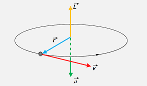So the electron orbit – in whatever way we’d want to visualize it – gives us L, which we refer to as the orbital angular momentum. We know the electron is also supposed to spin about its own axis – even if we know this planetary model of an electron isn’t quite correct. So that gives us a spin angular momentum S. In the so-called vector model of the atom, we simply add the two to get the total angular momentum J = L + S.

Of course, now you’ll say: only hydrogen has one electron, so how does it work with multiple electrons? Well… Then we have multiple orbital angular momentum l_i which are to be added to give a total orbital angular momentum L. Likewise, the electrons spins s_i can also be added to give some total spin angular momentum S. So we write:

J = L + S with L = Σ_i l_i and S = Σ_i s_i

Really? Well… If you’d google this to double-check – check the Wikipedia article on it, for example – then you’ll find this additivity property is valid only for relatively light atoms (Z ≤ 30) and only if any external magnetic field is weak enough. The way individual orbital and spin angular momenta have to be combined so as to arrive at some total L, S and J is referred to a coupling scheme: the additivity rule above is referred to as LS coupling, but one may also encounter LK coupling, or jj coupling, or other stuff. The US National Institute of Standards and Technology (NIST) has a nice article on all these models – but we need to move on here. Just note that we do assume the LS coupling scheme applies to our potassium beam – because its atomic number (Z) is 19, and the external magnetic field is assumed to be weak enough.

The vector model of the atom describes the atom using angular momentum vectors. Of course, we know that a magnetic field will cause our atomic magnet to precess – rather than line up. At this point, the classical analogy between a spinning top – or a gyroscope – and our atomic magnet becomes quite problematic. First, think about the implications for L and S when assuming,  as we usually do, that J precesses nicely about an axis that is parallel to the magnetic field – as shown in the illustration below, which I took from Feynman’s treatment of the matter. If J is the sum of two other vectors L and S, then this has rather weird implications for the precession of L and S, as shown in the illustration below – which I took from the Wikipedia article on LS coupling. Think about: if L and S are independent, then the axis of precession for these two vectors should be just the same as for J, right? So their axis of precession should also be parallel to the magnetic field (B), so that’s the direction of the J_z component, which is just the z-axis of our reference frame here.More importantly, our classical model also gets into trouble when actually measuring the magnitude of J_z: repeated measurements will not yield some randomly distributed continuous variable, as one would classically expect. No. In fact, that’s what this experiment is all about: it shows that J_z will take only certain quantized values. That is what is shown in the illustration below (which once again assumes the magnetic field (B) is along the z-axis). 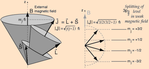I copied the illustration above from the HyperPhysics site, because I found it to be enlightening and intriguing at the same time. First, it also shows this rather weird implication of the vector model: if J continually changes direction because of its precession in a weak magnetic field, then L and S must, obviously, also continually change direction. However, this illustration is even more intriguing than the Wikipedia illustration because it assumes the axis of precession of L and S and L actually the same!

So what’s going on here? To better understand what’s going on, I started to read the whole HyperPhysics article on the vector model, which also includes the illustration below, with the following comments: “When orbital angular momentum L and electron spin S are combined to produce the total angular momentum of an atomic electron, the combination process can be visualized in terms of a vector model. Both the orbital and spin angular momenta are seen as precessing about the direction of the total angular momentum J. This diagram can be seen as describing a single electron, or multiple electrons for which the spin and orbital angular momenta have been combined to produce composite angular momenta S and L respectively. In so doing, one has made assumptions about the coupling of the angular momenta which are described by the LS coupling scheme which is appropriate for light atoms with relatively small external magnetic fields.”Hmm… What about those illustrations on the right-hand side – with the vector sums and those values for j and m_j? I guess the idea may also be illustrated by the table below: combining different values for l (±1) and s (±1/2) gives four possible values, ranging from +3/2 to -1/2, for j = l + s.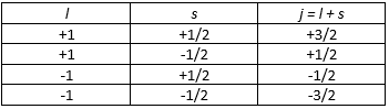Having said that, the illustration raises a very fundamental question: the length of the sum of two vectors is definitely not the same as the sum of the length of the two vectors! So… Well… Hmm… Something doesn’t make sense here! However, I can’t dwell any longer on this. I just wanted to note you should not take all that’s published on those oft-used sites on quantum mechanics for granted. But so I need to move on. Back to the other illustration – copied once more below.We have that very special formula for the magnitude (J) of the angular momentum J:

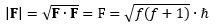
│J│= J = √(J·J) = √[j·(j+1)·ħ²] = √[j·(j+1)]·ħ 

So if j = 3/2, then J is equal to √[(3/2)·(3/2+1)]·ħ = √[(15/4)·ħ ≈ 1.9635·ħ, so that’s almost 2ħ. 🙂 At the same time, we know that for j = 3/2, the possible values of J_z can only be +3ħ/2, +ħ/2, -ħ/2, and -3ħ/2. So that’s what’s shown in that half-circular diagram: the magnitude of J is larger than its z-component – always!

OK. Next. What’s that 3p_3/2 notation? Excellent question! Don’t think this 3p denotes an electron orbital, like 1s or 3d – i.e. the orbitals we got from solving Schrödinger’s equation. No. In fact, the illustration above is somewhat misleading because the correct notation is not 3p_3/2 but ³P_3/2. So we have a capital P which is preceded by a superscript 3. This is the notation for the so-called term symbol for a nuclear, atomic or molecular (ground) state which – assuming our LS coupling model is valid – because we’ve got other term symbols for other coupling models – we can write, more generally, as:

^2S+1L_J

The J, L and S in this thing are the following:

1. The J is the total angular momentum quantum number, so it is – the notation gets even more confusing now – the j in the │J│= J = √(J·J) = √[j·(j+1)·ħ²] = √[j·(j+1)]·ħ expression. We know that number is 1/2 for electrons, but it may take on other values for nuclei, atoms or molecules. For example, it is 3/2 for nitrogen, and 2 for oxygen, for which the corresponding terms are ⁴S_3/2 and ³P₂ respectively.

2. The S in the term symbol is the total spin quantum number, and 2S+1 itself is referred to as the fine-structure multiplicity. It is not an easy concept. Just remember that the fine structure describes the splitting of the spectral lines of atoms due to electron spin. In contrast, the gross structure energy levels are those we effectively get from solving Schrödinger’s equation assuming our electrons have no spin.  We also have a hyperfine structure, which is due to the existence of a (small) nuclear magnetic moment, which we do not take into consideration here, which is why the ⁴S_3/2 and ³P₂ terms are sometimes being referred to as describing electronic ground states. In fact, the MIT lab document, which we are studying here, refers to the ground state of the potassium atoms in the beam as an electronic ground state, which is written up as ²S_1/2. So S is, effectively, equal to 1/2. [Are you still there? If so, just write it down: 2S+1 = 2 ⇒ S = 1/2. That means the following: our potassium atom behaves like an electron: its spin is either ‘up’ or, else, it is ‘down’. There is no in-between.]

3. Finally, the L in the term symbol is the total orbital angular momentum quantum number but, rather than using a number, the values of L are often represented as S, P, D, F, etcetera. This L number is very confusing because – as mentioned above – one would think it represents those s, p, d, f, g,… orbitals. However, that is not the case. The difference may easily be illustrated by observing that a carbon atom, for example, has six electrons, which are distributed over the 1s, 2s and 2p orbitals (one pair each). However, its ground state only gets one L number: L = P. Hence, its value is 1. Of course, now you will wonder how we get that number.

Well… I wish I could give you an easy answer, but I can’t. For two p electrons – think of our carbon atom once again – we can have L = 0, 1 or 2, or S, P and D. They effectively correspond to different energy levels, which are related to the way these two electrons interact with each other. The phenomenon is referred to as angular momentum coupling. In fact, all of the numbers we discussed so far – J, S and L – are numbers resulting from angular momentum coupling. As Wikipedia puts it: “Angular momentum coupling refers to the construction of eigenstates of total angular momentum out of eigenstates of separate angular momentum.” [As you know, each eigenstate corresponds to an energy level, of course.]

Now that should clear some of the confusion on the ^2S+1L_J notation: the capital letters J, S and L refer to some total, as opposed to the quantum numbers you are used to, i.e. n, l, m and s, i.e. the so-called principal, orbital, magnetic and spin quantum number respectively. The lowercase letters are quantum numbers that describe an electron in an atom, while those capital letters denote quantum numbers describing the atom – or a molecule – itself.

OK. Onwards. But where were we? 🙂 Oh… Yes. That J = L + S formula gives us some total electronic angular momentum, but we’ll also have some nuclear angular momentum, which our MIT paper denotes as I. Our vector model of our potassium atom allows us, once again, to simply add the two to get the total angular momentum, which is written as F = J + I = L + S + I. This, then, explains why the MIT experiment writes the magnitude of the total angular momentum as:

Of course, here I don’t need to explain – or so I hope – why this quantum-mechanical formula for the calculation of the magnitude is what it is (or, equivalently, why the usual Euclidean metric – i.e. √(x² + y² + z²) – is not to be used here. If you do need an explanation, you’ll need to go through the basics once again.

Now, the whole point, of course, is that the z-component of F can have only the discrete values that are specified by the F_z = m_f·ħ equation, with m_f – i.e. the (total) magnetic quantum number – having an equally discrete value equal to m_f = −f, −(f−1), …, +(f+1), f.

For the rest, I probably shouldn’t describe the experiment itself: you know it. But let me just copy the set-up below, so it’s clear what it is that we’re expecting to happen. In addition, you’ll also need the illustration below because I’ll refer to those d₁ and d₂ distances shown in what follows.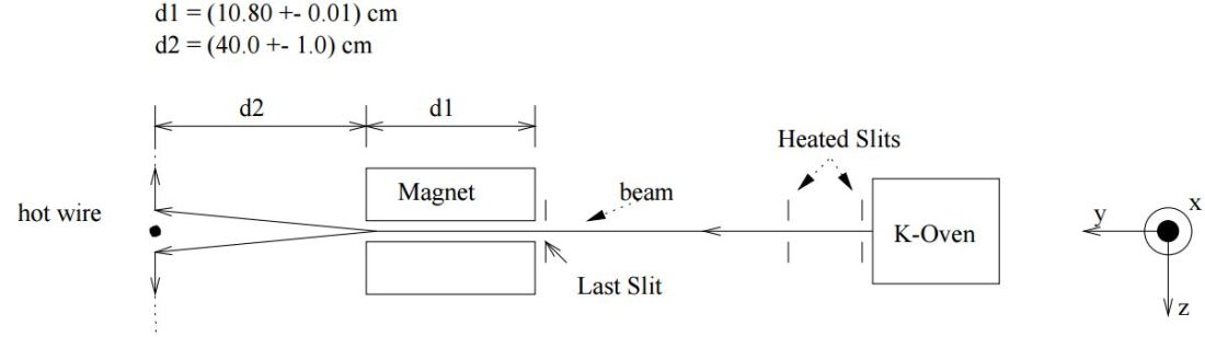

Note the MIT documentation does spell out some additional assumptions. Most notably, it says that the potassium atoms that emerge from the oven (at a temperature of 200°) will be:

(1) almost exclusively in the ground electronic state,

(2) nearly equally distributed among the two (magnetic) sub-states characterized by f, and, finally,

(3) very nearly equally distributed among the hyperfine states, i.e. the states with the same f but with different m_f.

I am just noting these assumptions because it is interesting to note that – according to the man or woman who wrote this paper – we would actually have states within states here. The paper states that the hyperfine splitting of the two sub-beams we expect to come out of the magnet can only be resolved by very advanced atomic beam techniques, so… Well… That’s not the apparatus that’s being used for this experiment.

However, it’s all a bit weird, because the paper notes that the rules for combining the electronic and nuclear angular momentum – using that F = J + I = L + S + I formula – imply that our quantum number f = i ± j can be either 1 or 2. These two values would be associated with the following m_f and m_f force values:

f = 1 ⇒ F_z = m_f·ħ = −ħ, 0 or +ħ (so we’d have three beams here)

f = 2 ⇒ F_z = m_f·ħ = −2ħ, −ħ, 0, +ħ or +2ħ (so we’d have five beams here)

Neither of the two possibilities relates to the situation at hand – which assumes two beams only. In short, I think the man or women who wrote the theoretical introduction – an assistant professor, most likely (no disrespect here: that’s how far I progressed in economics – nothing more, nothing less) – might have made a mistake. Or perhaps he or she may have wanted to confuse us.

I’ll look into it over the coming days. As for now, all you need to know – please jot it down! – is that our potassium atom is fully described by ²S_1/2. That shorthand notation has all the quantum number we need to know. Most importantly, it tells us S is, effectively, equal to 1/2. So… Well… That ²S_1/2 notation tells us our potassium atom should behave like an electron: its spin is either ‘up’ or ‘down’. No in-between. 🙂 So we should have two beams. Not three or five. No fine or hyperfine sub-structures! 🙂 In any case, the rest of the paper makes it clear the assumption is, effectively, that the angular momentum number is equal to j = 1/2. So… Two beams only. 🙂

How to calculate the expected deflection

We know that the inhomogeneous magnetic field (B), whose direction is the z-axis, will result in a force, which we have calculated a couple of times already as being equal to: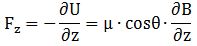In case you’d want to check this, you can check one of my posts on this. I just need to make one horrifying remark on notation here: while the same symbol is used, the force F_z is, obviously, not to be confused with the z-component of the angular momentum F = J + I = L + S + I that we described above. Frankly, I hope that the MIT guys have corrected that in the meanwhile, because it’s really terribly confusing notation! In any case… Let’s move on.

Now, we assume the deflecting force is constant because of the rather particular design of the magnet pole pieces (see Appendix I of the paper). We can then use Newton’s Second Law (F = m·a) to calculate the velocity in the z-direction, which is denoted by V_z (I am not sure why a capital letter is used here, but that’s not important, of course). That velocity is assumed to go from 0 to its final value V_z while our potassium atom travels between the two magnet poles but – to be clear – at any point in time, V_z will increase linearly – not exponentially – so we can write: V_z = a·t₁, with t₁ the time that is needed to travel through the magnet. Now, the relevant mass is the mass of the atom, of course, which is denoted by M. Hence, it is easy to see that a = F_z/M = V_z/t₁. Hence, we find that V_z = F_z·t₁/M.

Now, the vertical distance traveled (z) can be calculated by solving the usual integral: z = ∫₀^t₁ v(t)·dt = ∫₀^t₁ a·t·dt = a·t₁²/2 = (V_z/t₁)·t₁²/2 = V_z·t₁/2. Of course, once our potassium atom comes out of the magnetic field, it will continue to travel upward or downward with the same velocity V_z, which adds V_z·t₂ to the total distance traveled along the z-direction. Hence, the formula for the deflection is, effectively, the one that you’ll find in the paper:

z = V_z·t₁/2 + V_z·t₂ = V_z·(t₁/2 + t₂)

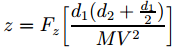
Now, the travel times depend on the velocity of our potassium atom along the y-axis, which is approximated by equating it with │V│= V, because the y-component of the velocity is easily the largest – by far! Hence, t₁ = d₁/V and t₂ = d₂/V. Some more manipulation will then give you the expression we need, which is a formula for the deflection in terms of variables that we actually know:

Statistical mechanics

We now need to combine this with the Maxwell-Boltzmann distribution for the velocities we gave you in our previous post: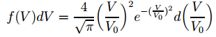The next step is to use this formula so as to be able to calculate a distribution which would describe the intensity of the beam. Now, it’s easy to understand such intensity will be related to the flux of potassium atoms, and it’s equally easy to get that a flux is defined as the rate of flow per unit area. Hmm… So how does this get us the formula below?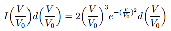The tricky thing – of course – is the use of those normalized velocities because… Well… It’s easy to see that the right-hand side of the equation above – just forget about the d(V/V₀ ) bit for a second, as we have it on both sides of the equation and so it cancels out anyway – is just density times velocity. We do have a product of the density of particles and the velocity with which they emerge here – albeit a normalized velocity. But then… Who cares? The normalization is just a division by V₀ – or a multiplication by 1/V₀, which is some constant. From a math point of view, it doesn’t make any difference: our variable is V/V₀ instead of V. It’s just like using some other unit. No worries here – as long as you use the new variable consistently everywhere. 🙂

Alright. […] What’s next? Well… Nothing much. The only thing that we still need to explain now is that factor 2. It’s easy to see that’s just a normalization factor – just like that 4/√π factor in the first formula. So we get it from imposing the usual condition: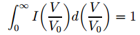So… What’s next… Well… We’re almost there. 🙂 As the MIT paper notes, the f(V) and I(V/V₀) functions can be mapped to each other: the related transformation maps a velocity distribution to an intensity distribution – i.e. a distribution of the deflection – and vice versa.

Now, the rest of the paper is just a lot of algebraic manipulations – distinguishing the case of a quantized F_z versus a continuous F_z. Here again, I must admit I am a bit shocked by the mix-up of concepts and symbols. The paper talks about a quantized deflecting force – while it’s obvious we should be talking a quantized angular momentum. The two concepts – and their units – are fundamentally different: the unit in which angular momentum is measured is the action unit: newton·meter·second (N·m·s). Force is just force: x newton.

Having said that, the mix-up does trigger an interesting philosophical question: what is quantized really? Force (expressed in N)? Energy (expressed in N·m)? Momentum (expressed in N·s)? Action (expressed in N·m·s, i.e. the unit of angular momentum)? Space? Time? Or space-time – related through the absolute speed of light (c)? Three factors (force, distance and time), six possibilities. What’s your guess?

[…]

What’s my guess? Well… The formulas tell us the only thing that’s quantized is action: Nature itself tells us we have to express it in terms of Planck units. However, because action is a product involving all of these factors, with different dimensions, the quantum-mechanical quantization of action can, obviously, express itself in various ways. 🙂

Some content on this page was disabled on June 16, 2020 as a result of a DMCA takedown notice from The California Institute of Technology. You can learn more about the DMCA here:

https://en.support.wordpress.com/copyright-and-the-dmca/