Statistical mechanics re-visited

Quite a while ago – in June and July 2015, to be precise – I wrote a series of posts on statistical mechanics, which included digressions on thermodynamics, Maxwell-Boltzmann, Bose-Einstein and Fermi-Dirac statistics (probability distributions used in quantum mechanics), and so forth. I actually thought I had sort of exhausted the topic. However, when going through the documentation on that Stern-Gerlach experiment that MIT undergrad students need to analyze as part of their courses, I realized I did actually not present some very basic formulas that you’ll definitely need in order to actually understand that experiment.

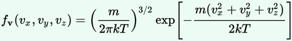
One of those basic formulas is the one for the distribution of velocities of particles in some volume (like an oven, for instance), or in a particle beam – like the beam of potassium atoms that is used to demonstrate the quantization of the magnetic moment in the Stern-Gerlach experiment. In fact, we’ve got two formulas here, which are subtly – as subtle as the difference between v (boldface, so it’s a vector) and v (lightface, so it’s a scalar) 🙂 – but fundamentally different:

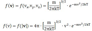
Both functions are referred to as the Maxwell-Boltzmann density distribution, but the first distribution gives us the density for some v in the velocity space, while the second gives us the distribution density of the absolute value (or modulus) of the velocity, so that is the distribution density of the speed, which is just a scalar – without any direction. As you can see, the second formula includes a 4π·v² factor.

The question is: how are these formulas related to Boltzmann’s f(E) = C·e^−energy/kT Law? The answer is: we can derive all of these formulas – for the distribution of velocities, or of momenta – by clever substitutions. However, as evidenced by the two formulas above, these substitutions are not always straightforward. So let me quickly show you a few things here.

First note the two formulas above already include the e^−energy/kT function if we equate the energy E with the kinetic energy: E = K.E. = m·v²/2. Of course, if you’ve read those June-July 2015 posts, you’ll note that we derived Boltzmann’s Law in the context of a force field, like gravity, or an electric potential. For example, we wrote the law for the density (n = N/V) of gas in a gravitational field (like the Earth’s atmosphere) as n = n₀·e^−P.E./kT. In this formula, we only see the potential energy: P.E. = m·g·h, i.e. the product of the mass (m), the gravitational constant (g), and the height (h). However, when we’re talking the distribution of velocities – or of momenta – then the kinetic energy comes into play.

So that’s a first thing to note: Boltzmann’s Law is actually a whole set of laws. For example, the frequency distribution of particles in a system over various possible states, also involves the same exponential function: F(state) ∝ e^−E/kT. E is just the total energy of the state here (which varies from state to state, of course), so we don’t distinguish between potential and kinetic energy here.

So what energy concept should we use in that Stern-Gerlach experiment? Because these potassium atoms in that oven – or when they come out of it in a beam – have kinetic energy only, our E = m·v²/2 substitution does the trick: we can say that the potential energy is taken to be zero, so that all energy is in the form of kinetic energy. So now we understand the e^−m·v2/2kT function in those f(v) and f(v) formulas. Now we only need to explain those complicated coefficients. How do we get these?

We get them through clever substitutions using equations such as:

f_v(v)·dv  = f_p(p)·dp

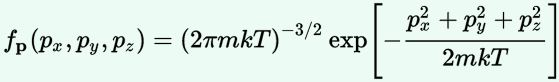
What are we writing here? We’re basically combining two normalization conditions: if f_v(v) and f_p(p) are proper probability density functions, then they must give us 1 when integrating over their domain. The domain of these two functions is, obviously, the velocity (v) and momentum (p) space. The velocity and momentum space are the same mathematical space, but they are obviously not the same physical space. But the two physical spaces are closely related: p = m·v, and so it’s easy to do the required transformation of variables. For example, it’s easy to see that, if E = m·v²/2, then E is also equal to E = p²/2m.

However, when doing these substitutions, things get tricky. We already noted that p and v are vectors, unlike E, or p and v – which are scalars, or magnitudes. So we write: p = (p_x, p_y, p_z) and |p| = p, and v = (v_x, v_y, v _z) and |v| = v. Of course, you also know how we calculate those magnitudes:

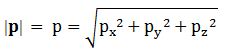
Note that this also implies the following: p·p = p² = p_x² + p_y² +p_z² = p². Trivial, right? Yes. But have a look now at the following differentials:

• d³p
• dp
• dp = d(p_x, p_y, p_z)
• dp_x·dp_y·dp_z

Are these the same or not? Now you need to think, right? That d³p and dp are different beasts is obvious: d³p is, obviously, some infinitesimal volume, as opposed to dp, which is, equally obviously, an (infinitesimal) interval. But what volume exactly? Is it the same as that dp = d(p_x, p_y, p_z) volume, and is that the same as the dp_x·dp_y·dp_z volume?

Fortunately, the volume differentials are, in fact, the same – so you can start breathing again. 🙂 Let’s get going with that d³p notation for the time being, as you will find that’s the notation which is used in the Wikipedia article on the Maxwell-Boltzmann distribution – which I warmly recommend, because – for a change – it is a much easier read than other Wikipedia articles on stuff like this. Among other things, the mentioned article writes the following:

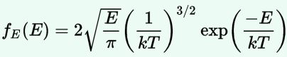
f_E(E)·dE = f_p(p)·d³p

What is this? Well… It’s just like that f_v(v)·dv  = f_p(p)·dp equation: it combines the normalization condition for both distributions. However, it’s much more interesting, because, on the left-hand side, we multiply a density with an (infinitesimal) interval (dE), while on the right-hand side we multiply with an (infinitesimal) volume (d³p). Now, the (infinitesimal) energy interval dE must, obviously, correspond with the (infinitesimal) momentum volume d³p. So how does that work?

Well… The mentioned Wikipedia article talks about the “spherical symmetry of the energy-momentum dispersion relation” (that dispersion relation is just E = |p|²/2m, of course), but that doesn’t make us all that wiser, so let’s try a more heuristic approach. You might remember the formula for the volume of a spherical shell, which is simply the difference between the volume of the outer sphere minus the volume of the inner sphere: V = (4π/3)·R³ − (4π/3)·r³ = (4π/3)·(R³ − r³). Now, for a very thin shell of thickness Δr, we can use the following first-order approximation: V = 4π·r²·Δr. In case you wonder, I hereby copy a nice explanation from the Physics Stack Exchange site:

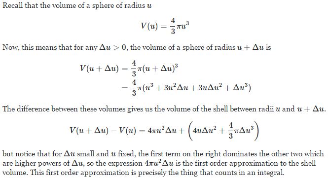
Perfect. That’s all we need to know. We’ll use that first-order approximation to re-write d³p as:

d³p = dp = 4π·|p|²·d|p| = 4π·p²·dp

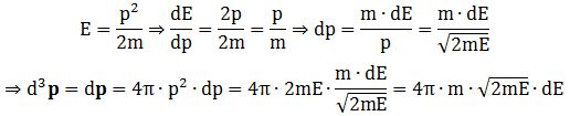
Note that we’ll have the same formula for d³v, of course: d³v = dv = 4π·|v|²·d|v| = 4π·v²·dv, and also note that we get that same 4π·v² factor which we mentioned when discussing the f(v) and f(v) formulas. That is not a coincidence, of course, but – as I’ll explain in a moment – it is not so easy to immediately relate the formulas. In any case, we’re now ready to relate dE and dp so we can re-write that d³p formula in terms of m, E and dE:

We are now – finally! – sufficiently armed to derive all of the formulas we want – or need. Let me just copy them from the mentioned Wikipedia article:

As said, you’ll encounter these formulas regularly – and so it’s good that you know how you can derive them. Indeed, the derivation is very straightforward and is done in the same article: the tips I gave you should allow you to read it in a couple of minutes only. Only the density function for velocities might cause you a bit of trouble – but only for a very short moment: just use the p = m·v equation to write d³p as d³p = 4π·p²·dp = 4π·m²·v²·m·dv = 4π·m³·v²·dv = m³·d³v, and you’re all set. 🙂

Of course, you will recognize the formula for the distribution of velocities: it’s the f(v) we mentioned in the introduction. However, you’re more likely to need the f(v) formula (i.e. the probability density function for the speed) than the f(v) function. So how can we derive get the f(v) – i.e. that formula for the distribution of speeds, with the 4π·v² factor – from the f(v) formula?

Well… I wish I could give you an easy answer. In fact, the same Wikipedia article suggests it’s easy – but it’s not. It involves a transformation from Cartesian to polar coordinates: the volume element dv_x·dv_y·dv_z is to be written as v²·sinθ·dv·dθ·dφ. And then… Well… Have a look at this link. 🙂 It involves a so-called Jacobian transformation matrix. If you want to know more about it, then I recommend you read some article on how to transform distribution functions: here’s a link to one of those, but you can easily google others. Frankly, as for now, I’d suggest you just accept the formula for f(v) as for now. 🙂 Let me copy it from the same article in a slightly different form: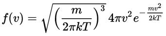Now, the final thing to note is that you’ll often want to use so-called normalized velocities, i.e. velocities that are defined as a v/v₀ ratio, with v₀ the most probable speed, which is equal to √(2kT/m). You get that value by calculating the df(v)/dv derivative, and then finding the value v = v₀ for which df(v)/dv = 0. You should now be able to verify the formula that is used in the mentioned MIT version of the Stern-Gerlach experiment: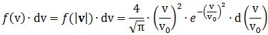Indeed, when you write it all out – note that π/π^3/2 = 1/√π 🙂 – you’ll see the two formulas are effectively equivalent. Of course, by now you are completely formula-ed out, and so you probably don’t even wonder what that f(v)·dv product actually stands for. What does it mean, really? Now you’ll sigh: why would I even want to know that? Well… I want you to understand that MIT experiment. 🙂 And you won’t if you don’t know what f(v)·dv actually represents. So think about it. […]

[…] OK. Let me help you once more. Remember the normalization condition once again: the integral of the whole thing – over the whole range of possible velocities – needs to add up to 1, so f(v)·dv is really the fraction of (potassium) atoms (inside the oven) with a velocity in the (infinitesimally small) dv interval. It’s going to be a tiny fraction, of course: just a tiny bit larger than zero. Surely not larger than 1, obviously. 🙂 Think of integrating the function between two values – say v₁ and v₂ – that are pretty close to each other.

So… Well… We’re done as for now. So where are we now in terms of understanding the calculations in that description of that MIT experiment? Well… We’ve got the meat. But we need a lot of other ingredients now. We’ll want formulas for the intensity of the beam at some point along the axis measuring its deflection from its main direction. That axis is the z-axis. So we’ll want a formula for some I(z) function.

Deflection? Yes. There are a lot of steps to go through now. Here’s the set-up: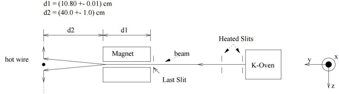First, we’ll need some formula measuring the flux of (potassium) atoms coming out of the oven. And then… Well… Just have a look and try to make your way through the whole thing now – which is just what I want to do in the coming days, so I’ll give you some more feedback soon. 🙂 Here I only wanted to introduce those formulas for the distribution of velocities and momenta, because you’ll need them in other contexts too.

So I hope you found this useful. Stuff like this all makes it somewhat more real, doesn’t it? 🙂 Frankly, I think the math is at least as fascinating as the physics. We could have a closer look at those distributions, for example, by noting the following:

1. The probability density function for the momenta is the product of three normal distributions. Which ones? Well…  The distribution of p_x, p_y and p_z respectively: three normal distributions whose variance is equal to mkT. 🙂

2. The f_E(E) function is a chi-squared (χ²) distribution with 3 degrees of freedom. Now, we have the equipartition theorem (which you should know – if you don’t, see my post on it), which tells us that this energy is evenly distributed among all three degrees of freedom. It is then relatively easy to show – if you know something about χ² distributions at least 🙂 – that the energy per degree of freedom (which we’ll write as ε below) will also be distributed as a chi-squared distribution with one degree of freedom: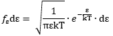This holds true for any number of degrees of freedom. For example, a diatomic molecule will have extra degrees of freedom, which are related to its rotational and vibrational motion (I explained that in my June-July 2015 posts too, so please go there if you’d want to know more). So we can really use this stuff in, for example, the theory of the specific heat of gases. 🙂

3. The function for the distribution of the velocities is also a product of three independent normally distributed variables – just like the density function for momenta. In this case, we have the v_x, v_y and v_z variables that are normally distributed, with variance kT/m.

So… Well… I’m done – for the time being, that is. 🙂 Isn’t it a privilege to be alive and to be able to savor all these little wonderful intellectual excursions? I wish you a very nice day and hope you enjoy stuff like this as much as I do. 🙂