Compactifying complex spaces

Pre-scriptum (dated 26 June 2020): the material in this post remains interesting but is, strictly speaking, not a prerequisite to understand quantum mechanics. It’s yet another example of how one can get lost in math when studying or teaching physics.

Original post:

In this post, I’ll try to explain how Riemann surfaces (or topological spaces in general) are transformed into compact spaces. Compact spaces are, in essence, closed and bounded subsets of some larger space. The larger space is unbounded – or ‘infinite’ if you want (the term ‘infinite’ is less precise – from a mathematical point of view at least).

I am sure you have all seen it: the Euclidean or complex plane gets wrapped around a sphere (the so-called Riemann sphere), and the Riemann surface of a square root function becomes a torus (i.e. a donut-like object). And then the donut becomes a coffee cup (yes: just type ‘donut and coffee cup’ and look at the animation). The sphere and the torus (and the coffee cup of course) are compact spaces indeed – as opposed to the infinite plane, or the infinite Riemann surface representing the domain of a (complex) square root function. But what does it all mean?

Let me, for clarity, start with a note on the symbols that I’ll be using in this post. I’ll use a boldface z for the complex number z = (x, y) = reⁱ^θin this post (unlike what I did in my previous posts, in which I often used standard letters for complex numbers), or for any other complex number, such as w = u + iv. That’s because I want to reserve the non-boldface letter z for the (real) vertical z coordinate in the three-dimensional (Cartesian or Euclidean) coordinate space, i.e. R³. Likewise, non-boldface letters such as x, y or u and v, denote other real numbers. Note that I will also use a boldface R and a boldface C to denote the set of real numbers and the complex space respectively. That’s just because the WordPress editor has its limits and, among other things, it can’t do blackboard bold (i.e. these double struck symbols which you usually see as symbols for the set of real and complex numbers respectively). OK. Let’s go for it now.

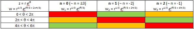
In my previous post, I introduced the concept of a Riemann surface using the multivalued square root function w = z^1/2= √z. The square root function has only two values. If we write z as z = reⁱ ^θ, then we can write these two values as w₁ = √r eⁱ⁽^θ/2)and w₂= √r eⁱ⁽^{θ/2 ± π)}. Now, √r eⁱ⁽^{θ/2 ± π)}is equal to √r eⁱ^(±π)eⁱ⁽^θ/2) = – √r eⁱ⁽^θ/2)and, hence, the second root is just the opposite of the first one, so w₂= – w₁.

Introducing the concept of a Riemann surface using a ‘simple’ quadratic function may look easy enough but, in fact, this square root function is actually not the easiest one to start with. First, a simple single-valued function, such as w = 1/z(i.e. the function that is associated with the Riemann sphere) for example, would obviously make for a much easier point of departure. Secondly, the fact that we’re working with a limited number of values, as opposed to an infinite number of values (which is the case for the log z function for example) introduces this particularity of a surface turning back into itself which, as I pointed out in my previous post, makes the visualization of the surface somewhat tricky – to the extent it may actually prevent a good understanding of what’s actually going on.

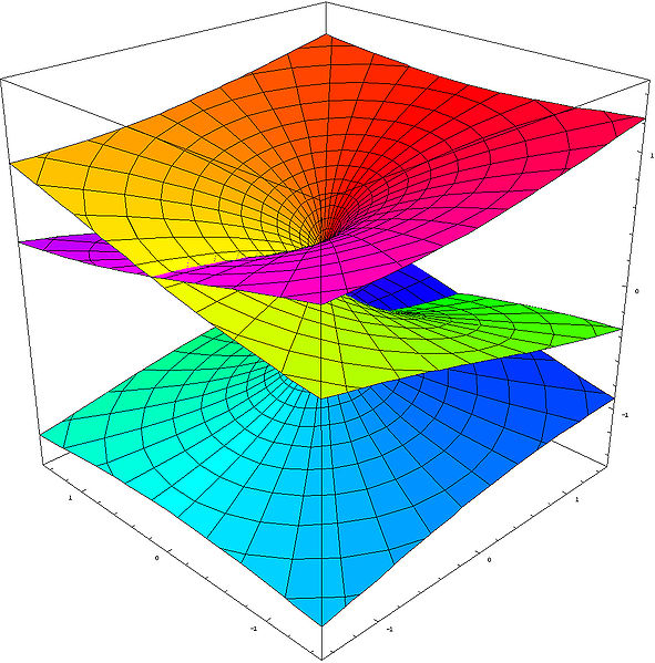
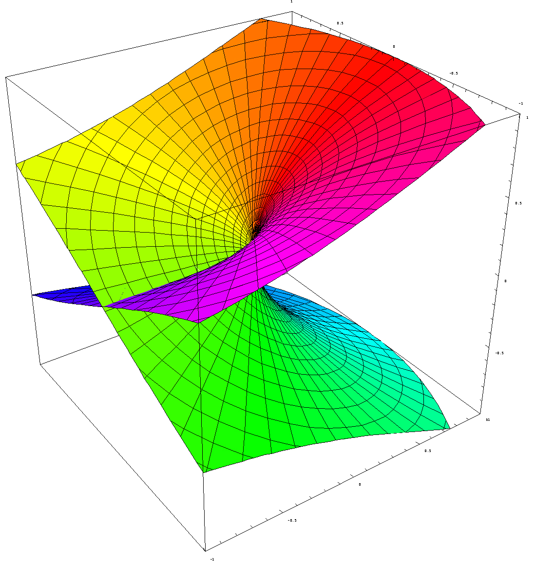
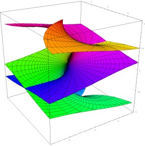
Indeed, in the previous post I explained how the Riemann surface of the square root function can be visualized in the three-dimensional Euclidean space (i.e. R³). However, such representations only show the real part of z^1/2, i.e. the vertical distance Re(z^1/2) = √r cos(θ/2 + nπ), with n = 0 or ± 1. So these representations, like the one below for example, do not show the imaginary part, i.e. Im(z^1/2) = √r sin(θ/2 + nπ) (n = 0, ± 1).

That’s both good and bad. It’s good because, in a graph like this, you want one point to represent one point only, and so you wouldn’t get that if you would superimpose the plot with the imaginary part of w = z^1/2on the plot showing the real part only. But it’s also bad, because one often forgets that we’re only seeing some part of the ‘real’ picture here, namely the real part, and so one often forgets to imagine the imaginary part. 🙂

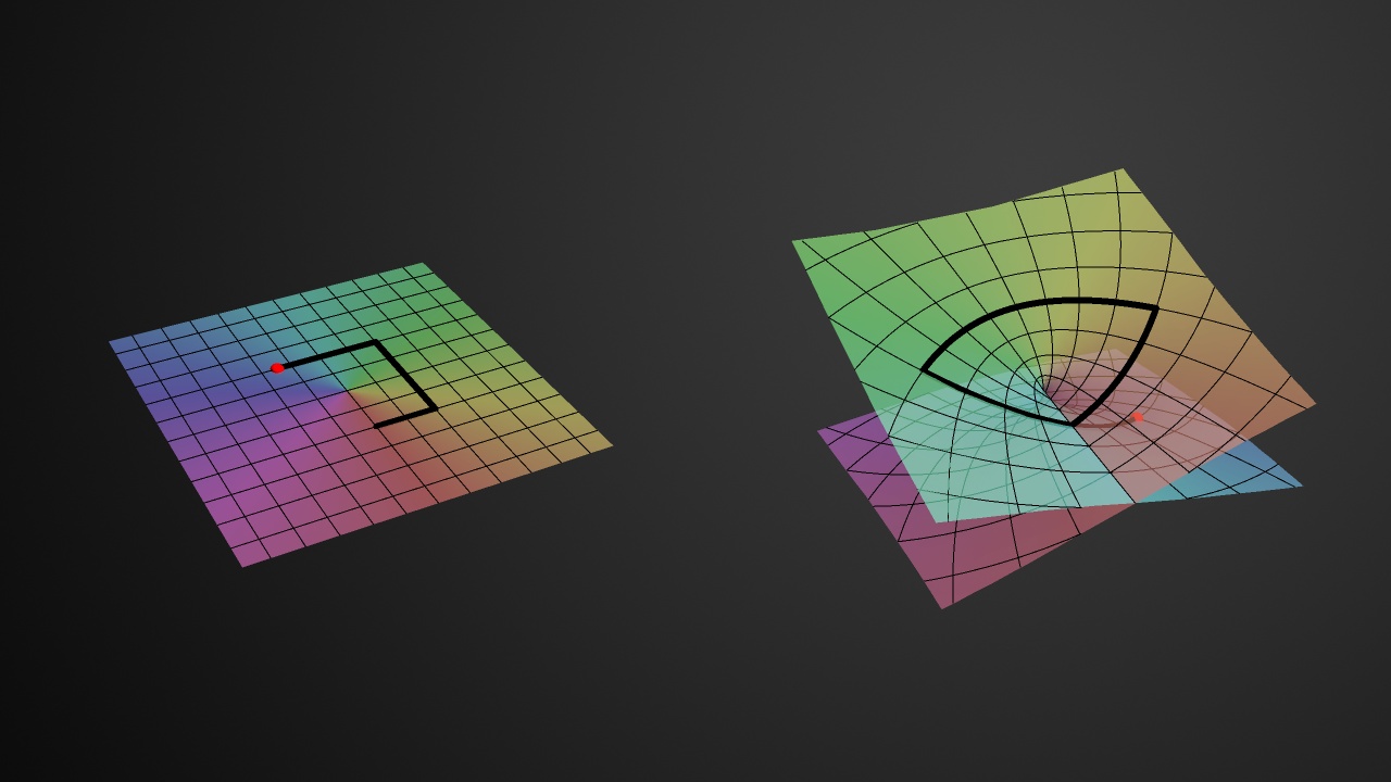
The thick black polygonal line in the two diagrams in the illustration above shows how, on this Riemann surface (or at least its real part), the argument θ of z = reⁱ ^θwill go from 0 to 2π (and further), i.e. we’re making (more than) a full turn around the vertical axis, as the argument Θ of w = z^1/2= √reⁱ^Θmakes half a turn only (i.e. Θ goes from 0 to π only). That’s self-evident because Θ = θ/2. [The first diagram in the illustration above represents the (flat) w plane, while the second one is the Riemann surface of the square root function, so it represents z but so we have like two points for every z on the flat z plane: one for each root.]

All these visualizations of Riemann surfaces (and the projections on the z and w plane that come with them) have their limits, however. As mentioned in my previous post, one major drawback is that we cannot distinguish the two distinct roots for all of the complex numbers z on the negative real axis (i.e. all the points z = reⁱ ^θfor which θ is equal to ±π, ±3π,…). Indeed, the real part of w = z^1/2, i.e. Re(w), is equal to zero for both roots there, and so, when looking at the plot, you may get the impression that we get the same values for w there, so that the two distinct roots of z (i.e. w₁and w₂) coincide. They don’t: the imaginary part of w₁and w₂is different there, so we need to look at the imaginary part of w too. Just to be clear on this: on the diagram above, it’s where the two sheets of the Riemann surface cross each other, so it’s like there’s an infinite number of branch points, which is not the case: the only branch point is the origin.

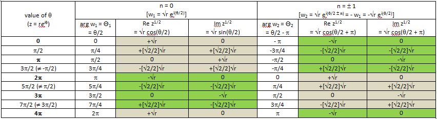
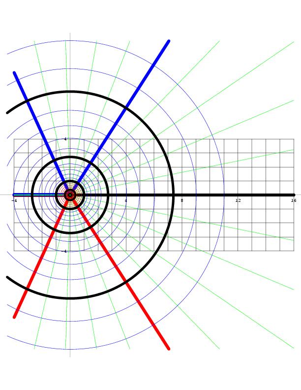
So we need to look at the imaginary part too. However, if we look at the imaginary part separately, we will have a similar problem on the positive real axis: the imaginary part of the two roots coincides there, i.e. Im(w) is zero, for both roots, for all the points z = reⁱ ^θfor which θ = 0, 2π, 4π,… That’s what represented and written in the graph below.

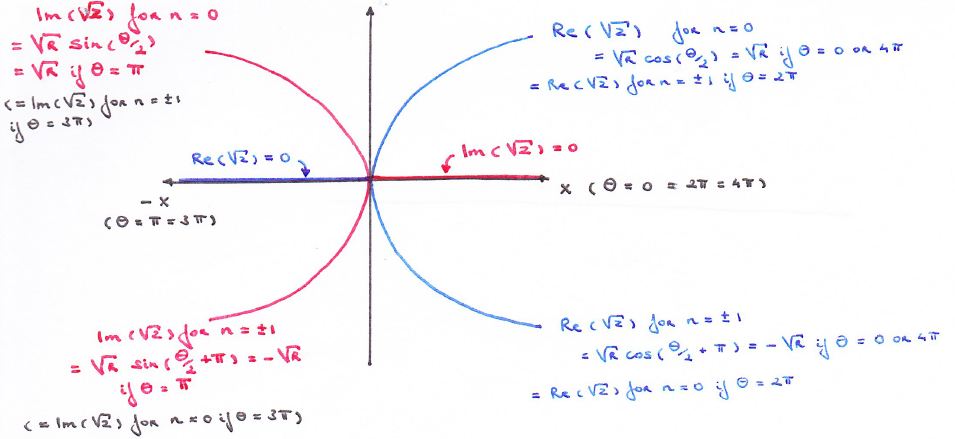
The graph above is a cross-section, so to say, of the Riemann surface w = z^1/2that is orthogonal to the z plane. So we’re looking at the x axis from -∞ to +∞ along the y axis so to say. The point at the center of this graph is the origin obviously, which is the branch point of our function w = z^1/2, and so the y axis goes through it but we can’t see it because we’re looking along that axis (so the y-axis is perpendicular to the cross-section).

This graph is one I made as I tried to get some better understanding of what a ‘branch point’ actually is. Indeed, the graph makes it perfectly clear – I hope 🙂 – that we really have to choose between one of the two branches of the function when we’re at the origin, i.e. the branch point. Indeed, we can pick either the n = 0 branch or the n = ±1 branch of the function, and then we can go in any direction we want as we’re traveling on that Riemann surface, but so our initial choice has consequences: as Dr. Teleman (whom I’ll introduce later) puts it, “any choice of w, followed continuously around the origin, leads, automatically, to the opposite choice as we turn around it.” For example, if we take the w₁branch (or the ‘positive’ root as I call it – even if complex numbers cannot be grouped into ‘positive’ or ‘negative’ numbers), then we’ll encounter the negative root w₂after one loop around the origin. Well… Let me immediately qualify that statement: we will still be traveling on the w₁branch but so the value of w₁will be the opposite or negative value of our original w₁as we add 2π to arg z = θ. Mutatis mutandis, we’re in a similar situation if we’d take the w₂branch. Does that make sense?

Perhaps not, but I can’t explain it any better. In any case, the gist of the matter is that we can switch from the w₁branch to the w₂branch at the origin, and also note that we can only switch like that there, at the branch point itself: we can’t switch anywhere else. So there, at the branch point, we have some kind of ‘discontinuity’, in the sense that we have a genuine choice between two alternatives.

That’s, of course, linked to the fact that one cannot define the value of our function at the origin: 0 is not part of the domain of the (complex) square root function, or of the (complex) logarithmic function in general (remember that our square root function is just a special case of the log function) and, hence, the function is effectively not analytic there. So it’s like what I said about the Riemann surface for the log z function: at the origin, we can ‘take the elevator’ to any other level, so to say, instead of having to walk up and down that spiral ramp to get there. So we can add or subtract ± 2nπ to θ without any sweat.

So here it’s the same. However, because it’s the square root function, we’ll only see two buttons to choose from in that elevator, and our choice will determine whether we get out at level Θ = α (i.e. the w₁branch) or at level Θ = α ± π (i.e. the w₂branch). Of course, you can try to push both buttons at the same time but then I assume that the elevator will make some kind of random choice for you. 🙂 Also note that the elevator in the log z parking tower will probably have a numpad instead of buttons, because there’s infinitely many levels to choose from. 🙂

OK. Let’s stop joking. The idea I want to convey is that there’s a choice here. The choice made determines whether you’re going to be looking at the ‘positive’ roots of z, i.e. √r(cosΘ+i sinΘ) or at the ‘negative’ roots of z, i.e. √r(cos(Θ±π)+isin(Θ±π)), or, equivalently (because Θ = θ/2) if you’re going to be looking at the values of w for θ going from 0 to 2π, or the values of w for θ going from 2π to 4π.

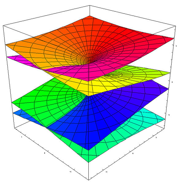
Let’s try to imagine the full picture and think about how we could superimpose the graphs of both the real and imaginary part of w. The illustration below should help us to do so: the blue and red image should be shifted over and across each other until they overlap completely. [I am not doing it here because I’d have to make one surface transparent so you can see the other one behind – and that’s too much trouble now. In addition, it’s good mental exercise for you to imagine the full picture in your head.]

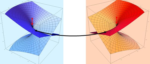
It is important to remember here that the origin of the complex z plane, in both images, is at the center of these cuboids (or ‘rectangular prisms’ if you prefer that term). So that’s what the little red arrow points is pointing at in both images and, hence, the final graph, consisting of the two superimposed surfaces (the imaginary and the real one), should also have one branch point only, i.e. at the origin.

[…]

I guess I am really boring my imaginary reader here by being so lengthy but so there’s a reason: when I first tried to imagine that ‘full picture’, I kept thinking there was some kind of problem along the whole x axis, instead of at the branch point only. Indeed, these two plots suggest that we have two or even four separate sheets here that are ‘joined at the hip’ so to say (or glued or welded or stitched together – whatever you want to call it) along the real axis (i.e. the x axis of the z plane). In such (erroneous) view, we’d have two sheets above the complex z plane (one representing the imaginary values of √z and one the real part) and two below it (again one with the values of the imaginary part of √z and one representing the values of the real part). All of these ‘sheets’ have a sharp fold on the x axis indeed (everywhere else they are smooth), and that’s where they join in this (erroneous) view of things.

Indeed, such thinking is stupid and leads nowhere: the real and imaginary parts should always be considered together, and so there’s no such thing as two or four sheets really: there is only one Riemann surface with two (overlapping) branches. You should also note that where these branches start or end is quite arbitrary, because we can pick any angle α to define the starting point of a branch. There is also only one branch point. So there is no ‘line’ separating the Riemann surface into two separate pieces. There is only that branch point at the origin, and there we decide what branch of the function we’re going to look at: the n = 0 branch (i.e. we consider arg w = Θ to be equal to θ/2) or the n = ±1 branch (i.e. we take the Θ = θ/2 ± π equation to calculate the values for w = z^1/2).

OK. Enough of these visualizations which, as I told you above already, are helpful only to some extent. Is there any other way of approaching the topic?

Of course there is. When trying to understand these Riemann surfaces (which is not easy when you read Penrose because he immediately jumps to Riemann surfaces involving three or more branch points, which makes things a lot more complicated), I found it useful to look for a more formal mathematical definition of a Riemann surface. I found such more formal definition in a series of lectures of a certain Dr. C. Teleman (Berkeley, Lectures on Riemann surfaces, 2003). He defines them as graphs too, or surfaces indeed, just like Penrose and others, but, in contrast, he makes it very clear, right from the outset, that it’s really the association (i.e. the relation) between z and w which counts, not these rather silly attempts to plot all these surfaces in three-dimensional space.

Indeed, according to Dr. Teleman’s introduction to the topic, a Riemann surface S is, quite simply, a set of ‘points’ (z, w) in the two-dimensional complex space C²= C x C (so they’re not your typical points in the complex plane but points with two complex dimensions), such that w and z are related with each other by a holomorphic function w = f(z), which itself defines the Riemann surface. The same author also usefully points out that this holomorphic function is usually written in its implicit form, i.e. as P(z, w) = 0 (in case of a polynomial function) or, more generally, as F(z, w) = 0.

There are two things you should note here. The first one is that this eminent professor suggests that we should not waste too much time by trying to visualize things in the three-dimensional R³= R x R x R space: Riemann surfaces are complex manifolds and so we should tackle them in their own space, i.e. the complex C²space. The second thing is linked to the first: we should get away from these visualizations, because these Riemann surfaces are usually much and much more complicated than a simple (complex) square root function and, hence, are usually not easy to deal with. That’s quite evident when we consider the general form of the complex-analytical (polynomial) P(z, w) function above, which is P(z, w) = wⁿ + p_n-1(z)w^n-1 + … + p₁(z)w + p₀(z), with the p_k(z) coefficients here being polynomials in z themselves.

That being said, Dr. Teleman immediately gives a ‘very simple’ example of such function himself, namely w = [(z²– 1) + ((z²– k²)]^1/2. Huh? If that’s regarded as ‘very simple’, you may wonder what follows. Well, just look him up I’d say: I only read the first lecture and so there are fourteen more. 🙂

But he’s actually right: this function is not very difficult. In essence, we’ve got our square root function here again (because of the ^1/2 exponent), but with four branch points this time, namely ± 1 and ± k (i.e. the positive and negative square roots of 1 and k²respectively, cf. the (z²– 1) and (z²– k²) terms in the argument of this function), instead of only one (the origin).

Despite the ‘simplicity’ of this function, Dr. Teleman notes that “we cannot identify this shape by projection (or in any other way) with the z-plane or the w-plane”, which confirms the above: Riemann surfaces are usually not simple and, hence, these ‘visualizations’ don’t help all that much. However, while not ‘identifying the shape’ of this particular square root function, Dr. Teleman does make the following drawing of the branch points:

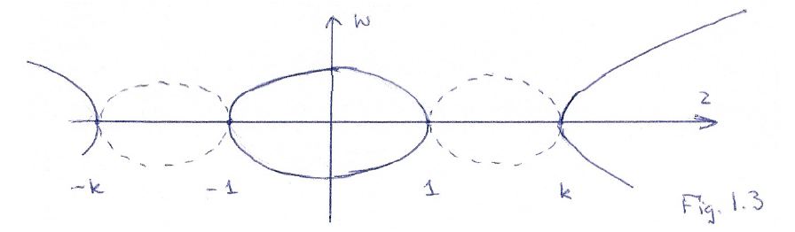
This is also some kind of cross-section of the Riemann surface, just like the one I made above for the ‘super-simple’ w = √z function: the dotted lines represent the imaginary part of w = [(z²– 1) + (z²– k²)]^1/2, and the non-dotted lines are the real part of the (double-valued) w function. So that’s like ‘my’ graph indeed, except that we’ve got four branch points here, so we can make a choice between one of the two branches of w at each of them.

[Note that one obvious difficulty in the interpretation of Dr. Teleman’s little graph above is that we should not assume that the complex numbers k and –k are actually lying on the same line as 1 and -1 (i.e. the real line). Indeed, k and –k are just standard complex numbers and most complex numbers do not lie on the real line. While that makes the interpretation of that simple graph of Dr. Teleman somewhat tricky, it’s probably less misleading than all these fancy 3D graphs. In order to proceed, we can either assume that this z axis is some polygonal line really, representing line segments between these four branch points or, even better, I think we should just accept the fact we’re looking at the z plane here along the z plane itself, so we can only see it as a line and we shouldn’t bother about where these points k and –k are located. In fact, their absolute value may actually be smaller than 1, in which case we’d probably want to change the order of the branch points in Dr. Teleman’s little graph).]

Dr. Teleman doesn’t dwell too long on this graph and, just like Penrose, immediately proceeds to what’s referred to as the compactification of the Riemann space, so that’s this ‘transformation’ of this complex surface into a donut (or a torus as it’s called in mathematics). So how does one actually go about that?

Well… Dr. Teleman doesn’t waste too many words on that. In fact, he’s quite cryptic, although he actually does provide much more of an explanation than Penrose does (Penrose’s treatment of the matter is really hocus-pocus I feel). So let me start with a small introduction of my own once again.

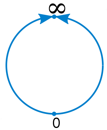
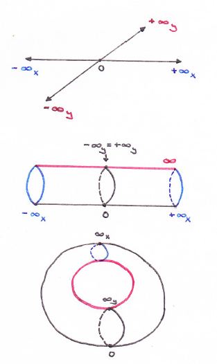
I guess it all starts with the ‘compactification’ of the real line, which is visualized below: we reduce the notion of infinity to a ‘point’ (this ‘point’ is represented by the symbol ∞ without a plus or minus sign) that bridges the two ‘ends’ of the real line (i.e. the positive and negative real half-line). Like that, we can roll up single lines and, by extension, the whole complex plane (just imagine rolling up the infinite number of lines that make up the plane I’d say :-)). So then we’ve got an infinitely long cylinder.

But why would we want to roll up a line, or the whole plane for that matter? Well… I don’t know, but I assume there are some good reasons out there: perhaps we actually do have some thing going round and round, and so then it’s probably better to transform our ‘real line’ domain into a ‘real circle’ domain. The illustration below shows how it works for a finite sheet, and I’d also recommend my imaginary reader to have a look at the Riemann Project website (http://science.larouchepac.com/riemann/page/23), where you’ll find some nice animations (but do download Wolfram’s browser plugin if your Internet connection is slow: downloading the video takes time). One of the animations shows how a torus is, indeed, ideally suited as a space for a phenomenon characterized by two “independent types of periodicity”, not unlike the cylinder, which is the ‘natural space’ for “motion marked by a single periodicity”.

However, as I explain in a note below this post, the more natural way to roll or wrap up a sheet or a plane is to wrap it around a sphere, rather than trying to create a donut. Indeed, if we’d roll the infinite plane up in a donut, we’ll still have a line representing infinity (see below) and so it looks quite ugly: if you’re tying ends up, it’s better you tie all of them up, and so that’s what you do when you’d wrap the plane up around a sphere, instead of a torus.

OK. Enough on planes. Back to our Riemann surface. Because the square root function w has two values for each z, we cannot make a simple sphere: we have to make a torus. That’s because a sphere has one complex dimension only, just like a plane, and, hence, they are topologically equivalent so to say. In contrast, a double-valued function has two ‘dimensions’ so to say and, hence, we have to transform the Riemann surface into something which accommodates that, and so that’s a torus (or a coffee cup :-)). In topological jargon, a torus has genus one, while the complex plane (and the Riemann sphere) has genus zero.

[Please do note that this will be the case regardless of the number of branch points. Indeed, Penrose gives the example of the function w = (1 – z³)^1/2, which has three branch points, namely the three cube roots of the 1 – z³expression (these three roots are obviously equal to the three cube roots of unity). However, ‘his’ Riemann surface is also a Riemann surface of a square root function (albeit one with a more complicated form than the ‘core’ w = z^1/2 example) and, hence, he also wraps it up as a donut indeed, instead of a sphere or something else.]

I guess that you, my imaginary reader, have stopped reading all of this nonsense. If you haven’t, you’re probably thinking: why don’t we just do it? How does it work? What’s the secret?

Frankly, the illustration in Penrose’s Road to Reality (i.e. Fig. 8.2 on p. 137) is totally useless in terms of understanding how it’s being done really. In contrast, Dr. Teleman is somewhat more explicit and so I’ll follow him here as much as I can while I try to make sense of it (which is not as easy as you might think).

The short story is the following: Dr. Teleman first makes two ‘cuts’ (or ‘slits’) in the z plane, using the four branch points as the points where these ‘cuts’ start and end. He then uses these cuts to form two cylinders, and then he joins the ends of these cylinders to form that torus. That’s it. The drawings below illustrate the proceedings.

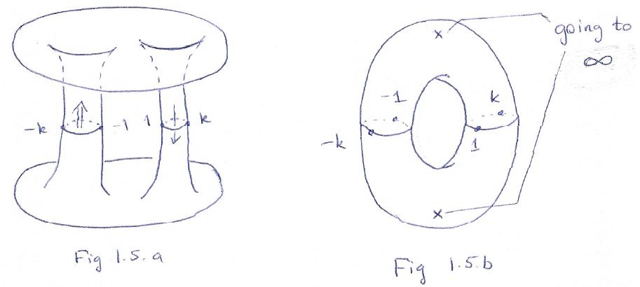
Huh? OK. You’re right: the short story is not correct. Let’s go for the full story. In order to be fair to Dr. Teleman, I will literally copy all what he writes on what is illustrated above, and add my personal comments and interpretations in square brackets (so when you see those square brackets, that’s [me] :-)). So this is what Dr. Teleman has to say about it:

The function w = [(z²– 1) + ((z²– k²)]^1/2 behaves like the [simple] square root [function] near ± 1 and ± k. The important thing is that there is no continuous single-valued choice of w near these points [shouldn’t he say ‘on’ these points, instead of ‘near’?]: any choice of w, followed continuously round any of the four points, leads to the opposite choice upon return.

[The formulation may sound a bit weird, but it’s the same as what happens on the simple w = z^1/2 surface: when we’re on one of the two branches, the argument of w changes only gradually and, going around the origin, starting from one root of z (let’s say the ‘positive’ root w₁), we arrive, after one full loop around the origin on the z plane (i.e. we add 2π to arg z = θ), at the opposite value, i.e. the ‘negative’ root w₂= -w₁.]

Defining a continuous branch for the function necessitates some cuts. The simplest way is to remove the open line segments joining 1 with k and -1 with –k. On the complement of these segments [read: everywhere else on the z plane], we can make a continuous choice of w, which gives an analytic function (for z ≠ ±1, ±k). The other branch of the graph is obtained by a global change of sign. [Yes. That’s obvious: the two roots are each other’s opposite (w₂= –w₁) and so, yes, the two branches are, quite simply, just each other’s opposite.]

Thus, ignoring the cut intervals for a moment, the graph of w breaks up into two pieces, each of which can be identified, via projection, with the z-plane minus two intervals (see Fig. 1.4 above). [These ‘projections’ are part and parcel of this transformation business it seems. I’ve encountered more of that stuff and so, yes, I am following you, Dr. Teleman!]

Now, over the said intervals [i.e. between the branch points], the function also takes two values, except at the endpoints where those coincide. [That’s true: even if the real parts of the two roots are the same (like on the negative real axis for our w = z^1/2 s), the imaginary parts are different and, hence, the roots are different for points between the various branch points, and vice versa of course. This is actually one of the reasons why I don’t like Penrose’s illustration on this matter: his illustration suggests that this is not the case.]

To understand how to assemble the two branches of the graph, recall that the value of w jumps to its negative as we cross the cuts. [At first, I did not get this, but so it’s the consequence of Dr. Teleman ‘breaking up the graph into tow pieces’. So he separates the two branches indeed, and he does so at the ‘slits’ he made, so that’s between the branch points. It follows that the value of w will indeed jump to its opposite value as we cross them, because we’re jumping on the other branch there.]

Thus, if we start on the upper sheet and travel that route, we find ourselves exiting on the lower sheet. [That’s the little arrows on these cuts.] Thus, (a) the far edges of the cuts on the top sheet must be identified with the near edges of the cuts on the lower sheet; (b) the near edges of the cuts on the top sheet must be identified with the far edges on the lower sheet; (c) matching endpoints are identified; (d) there are no other identifications. [Point (d) seems to be somewhat silly but I get it: here he’s just saying that we can’t do whatever we want: if we glue or stitch or weld all of these patches of space together (or should I say copies of patches of space?), we need to make sure that the points on the edges of these patches are the same indeed.]

A moment’s thought will convince us that we cannot do all this in in R³, with the sheets positioned as depicted, without introducing spurious crossings. [That’s why Brown and Churchill say it’s ‘physically impossible.’] To rescue something, we flip the bottom sheet about the real axis.

[Wow! So that’s the trick! That’s the secret – or at least one of them! Flipping the sheet means rotating it by 180 degrees, or multiplying all points twice with i, so that’s i²= -1 and so then you get the opposite values. Now that’s a smart move!]

The matching edges of the cuts are now aligned, and we can perform the identifications by stretching each of the surfaces around the cut to pull out a tube. We obtain a picture representing two planes (ignore the boundaries) joined by two tubes (see Fig. 1.5.a above).

[Hey! That’s like the donut-to-coffee-cup animation, isn’t it? Pulling out a tube? Does that preserve angles and all that? Remember it should!]

For another look at this surface, recall that the function z → R²/z identifies the exterior of the circle ¦z¦ < R with the punctured disc z: ¦z¦ < R and z ≠ 0 (it’s a punctured disc so its center is not part of the disc). Using that, we can pull the exteriors of the discs, missing from the picture above, into the picture as punctured discs, and obtain a torus with two missing points as the definitive form of our Riemann surface (see Fig. 1.5.b).

[Dr. Teleman is doing another hocus-pocus thing here. So we have those tubes with an infinite plane hanging on them, and so it’s obvious we just can’t glue these two infinite planes together because it wouldn’t look like a donut 🙂. So we first need to transform them into something more manageable, and so that’s the punctured discs he’s describing. I must admit I don’t quite follow him here, but I can sort of sense – a little bit at least – what’s going on.]

[…]

Phew! Yeah, I know. My imaginary reader will surely feel that I don’t have a clue of what’s going on, and that I am actually not quite ready for all of this high-brow stuff – or not yet at least. He or she is right: my understanding of it all is rather superficial at the moment and, frankly, I wish either Penrose or Teleman would explain this compactification thing somewhat better. I also would like them to explain why we actually need to do this compactification thing, why it’s relevant for the real world.

Well… I guess I can only try to move forward as good as I can. I’ll keep you/myself posted.

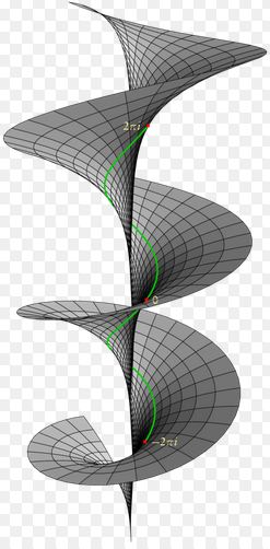
Note: As mentioned above, there is more than one way to roll or wrap up the complex plane, and the most natural way of doing this is to do it around a sphere, i.e. the so-called Riemann sphere, which is illustrated below. This particular ‘compactification’ exercise is equivalent to a so-called stereographic projection: it establishes a one-on-one relationship between all points on the sphere and all points of the so-called extended complex plane, which is the complex plane plus the ‘point’ at infinity (see my explanation on the ‘compactification’ of the real line above).

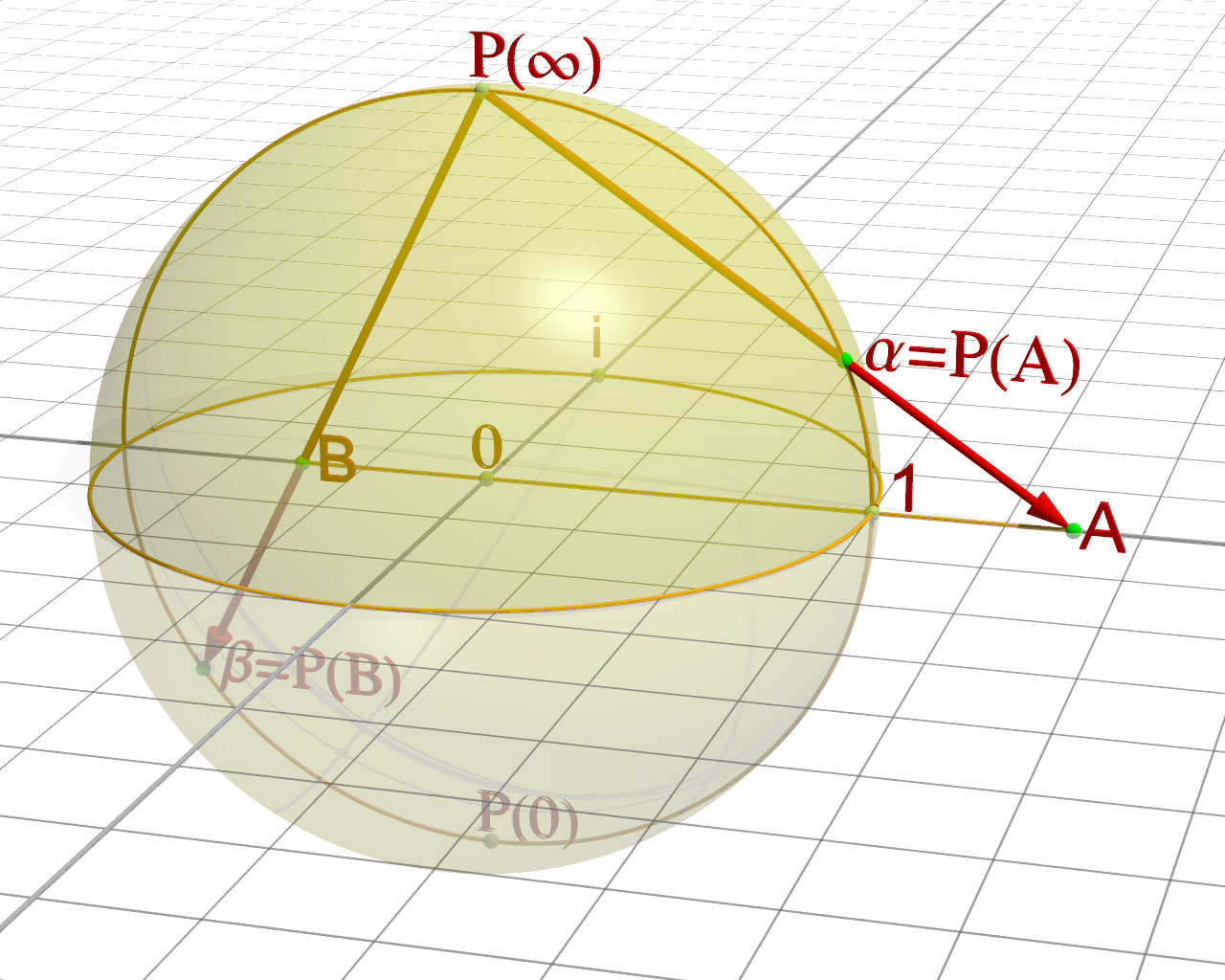
But so Riemann surfaces are associated with complex-analytic functions, right? So what’s the function? Well… The function with which the Riemann sphere is associated is w = 1/z. [1/z is equal to z = z*/¦z¦², with z* = x – iy, i.e. the complex conjugate of z = x + iy, and ¦z¦ the modulus or absolute value of z, and so you’ll recognize the formulas for the stereographic projection here indeed.]

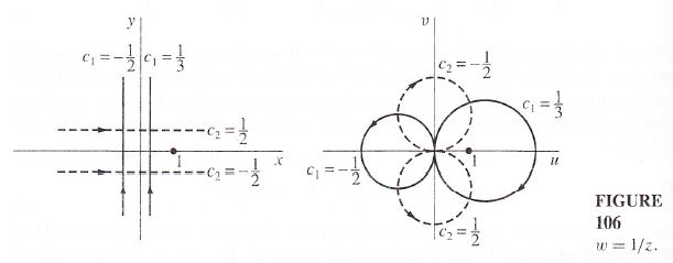
OK. So what? Well… Nothing much. This mapping from the complex z plane to the complex w plane is conformal indeed, i.e. it preserves angles (but not areas) and whatever else that comes with complex analyticity. However, it’s not as straightforward as Penrose suggests. The image below (taken from Brown and Churchill) shows what happens to lines parallel to the x and y axis in the z plane respectively: they become circles in the w plane. So this particular function actually does map circles to circles (which is what holomorphic functions have to do) but only if we think of straight lines as being particular cases of circles, namely circles “of infinite radius”, as Penrose puts it.

Frankly, it is quite amazing what Penrose expects in terms of mental ‘agility’ of the reader. Brown and Churchill are much more formal in their approach (lots of symbols and equations I mean, and lots of mathematical proofs) but, to be honest, I find their stuff easier to read, even if their textbook is a full-blown graduate level course in complex analysis.

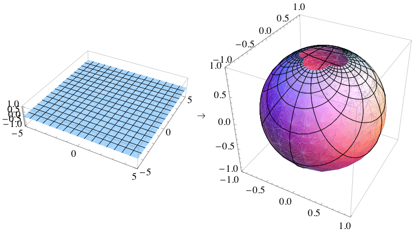
I’ll conclude this post here with two more graphs: they give an idea of how the Cartesian and polar coordinate spaces can be mapped to the Riemann sphere. In both cases, the grid on the plane appears distorted on the sphere: the grid lines are still perpendicular, but the areas of the grid squares shrink as they approach the ‘north pole’.

The mathematical equations for the stereographic projection, and the illustration above, suggest that the w = 1/z function is basically just another way to transform one coordinate system into another. But then I must admit there is a lot of finer print that I don’t understand – as yet that is. It’s sad that Penrose doesn’t help out very much here.

Riemann surfaces (II)

Original post:

This is my second post on Riemann surfaces, so they must be important. [At least I hope so, because it takes quite some time to understand them. :-)]

From my first post on this topic, you may or may not remember that a Riemann surface is supposed to solve the problem of multivalued complex functions such as, for instance, the complex logarithmic function (log z = ln r + i(θ + 2nπ) or the complex exponential function (z^c = e^{c log z}). [Note that the problem of multivaluedness for the (complex) exponential function is a direct consequence of its definition in terms of the (complex) logarithmic function.]

In that same post, I also wrote that it all looked somewhat fishy to me: we first use the function causing the problem of multivaluedness to construct a Riemann surface, and then we use that very same surface as a domain for the function itself to solve the problem (i.e. to reduce the function to a single-valued (analytic) one). Penrose does not have any issues with that though. In Chapter 8 (yes, that’s where I am right now: I am moving very slowly on his Road to Reality, as it’s been three months of reading now, and there are 34 chapters!), he writes that “Complex (analytic) functions have a mind of their own, and decide themselves what their domain should be, irrespective of the region of the complex plane which we ourselves may initially have allotted to it. While we may regard the function’s domain to be represented by the Riemann surface associated with the function, the domain is not given ahead of time: it is the explicit form of the function itself that tells us which Riemann surface the domain actually is.”

Let me retrieve the graph of the Riemannian domain for the log z function once more:

For each point z in the complex plane (and we can represent z both with rectangular as well as polar coordinates: z = x + iy = re^iθ), we have an infinite number of log z values: one for each value of n in the log z = ln r + i(θ + 2nπ) expression (n = 0, ±1, ±2, ±3,…, ±∞). So what we do when we promote this Riemann surface as a domain for the log z function is equivalent to saying that point z is actually not one single point z with modulus r and argument θ + 2nπ, but an infinite collection of points: these points all have the same modulus ¦z¦ = r but we distinguish the various ‘representations’ of z by treating θ, θ ± 2π, θ ±+ 4π, θ ± 6π, etcetera, as separate argument values as we go up or down on that spiral ramp. So that is what is represented by that infinite number of sheets, which are separated from each other by a vertical distance of 2π. These sheets are all connected at or through the origin (at which the log z function is undefined: therefore, the origin is not part of the domain), which is the branch point for this function. Let me copy some formal language on the construction of that surface here:

“We treat the z plane, with the origin deleted, as a thin sheet R₀which is cut along the positive half of the real axis. On that sheet, let θ range from 0 to 2π. Let a second sheet R₁be cut in the same way and placed in front of the sheet R₀. The lower edge of the slit in R₀is then joined to the upper edge of the slit in R₁. On R₁, the angle θ ranges from 2π to 4π; so, when z is represented by a point on R₁, the imaginary component of log z ranges from 2π to 4π.” And then we repeat the whole thing, of course: “A sheet R₂is then cut in the same way and placed in front of R₁. The lower edge of the slit in R₁. is joined to the upper edge of the slit in this new sheet, and similarly for sheets R₃, R₄… A sheet R_-1, R_-2, R_-3,… are constructed in like manner.” (Brown and Churchill, Complex Variables and Applications, 7th edition, p. 335-336)

The key phrase above for me is this “when z is represented by a point on R₁“, because that’s what it is really: we have an infinite number of representations of z here, namely one representation of z for each branch of the log z function. So, as n = 0, ±1, , ±2, ±3 etcetera, we have an infinite number of them indeed. You’ll also remember that each branch covers a range from some random angle α to α + 2π. Imagine a continuous curve around the origin on this Riemann surface: as we move around, the angle of z changes from 0 to 2θ on sheet R₀, and then from 2π to 4π on sheet R₁and so on and so on.

The illustration above also illustrates the meaning of a branch point. Imagine yourself walking on that surface and approaching the origin, from any direction really. At the origin itself, you can choose what to do: either you take the elevator up or down to some other level or, else, the elevator doesn’t work and so then you have to walk up or down that ramp to get to another level. If you choose to walk along the ramp, the angle θ changes gradually or, to put it in mathematical terms, in a continuous way. However, if you took the elevator and got out at some other level, you’ll find that you’ve literally ‘jumped’ one or more levels. Indeed, remember that log z = ln r + i(θ + 2nπ) and so ln r, the horizontal distance from the origin didn’t change, but you did add some multiple of 2π to the vertical distance, i.e. the imaginary part of the log z value.

Let us now construct a Riemann surface for some other multiple-valued functions. Let’s keep it simple and start with the square root of z, so c = 1/2, which is nothing else than a specific example of the complex exponential function z^c = z^c = e^{c log z}: we just take a real number for c here. In fact, we’re taking a very simple rational number value for c: 1/2 = 0.5. Taking the square, cube, fourth or n^th root of a complex number is indeed nothing but a special case of the complex exponential function. The illustration below (taken from Wikipedia) shows us the Riemann surface for the square root function.

As you can see, the spiraling surface turns back into itself after two turns. So what’s going on here? Well… Our multivalued function here does not have an infinite number of values for each z: it has only two, namely √r e^i(θ/2)and √r e^{i(θ/2 + π)}. But what’s that? We just said that the log function – of which this function is a special case – had an infinite number of values? Well… To be somewhat more precise: z^1/2actually does have an infinite number of values for each z (just like any other complex exponential function), but it has only two values that are different from each other. All the others coincide with one of the two principal ones. Indeed, we can write the following:

w = √z = z^1/2= e^{(1/2) log z}= e^{(1/2)[ln r + i(θ + 2nπ)]}= r^1/2e^{i(θ/2 + nπ)}= √re^{i(θ/2 + nπ)}

(n = 0, ±1, ±2, ±3,…)

For n = 0, this expression reduces to z^1/2= √re^iθ/2. For n = ±1, we have z^1/2= √re^{i(θ/2 + π)}, which is different than the value we had for n = 0. In fact, it’s easy to see that this second root is the exact opposite of the first root: √re^{i(θ/2 + π)} = √re^iθ/2e^iπ = – √re^iθ/2). However, for n = 2, we have z^1/2= √re^{i(θ/2 + 2π)}, and so that’s the same value (z^1/2= √re^iθ/2) as for n = 0. Indeed, taking the value of n = 2 amounts to adding 2π to the argument of w and so get the same point as the one we found for n = 0. [As for the plus or minus sign, note that, for n = -1, we have z^1/2= √re^{i(θ/2 -π)}= √re^{i(θ/2 -π+2π)}= √re^{i(θ/2 +π)}and, hence, the plus or minus sign for n does not make any difference indeed.]

In short, as mentioned above, we have only two different values for w = √z = z^1/2and so we have to construct two sheets only, instead of an infinite number of them, like we had to do for the log z function. To be more precise, because the sheet for n = ±2 will be the same sheet as for n = 0, we need to construct one sheet for n = 0 and one sheet for n = ±1, and so that’s what shown above: the surface has two sheets (one for each branch of the function) and so if we make two turns around the origin (one on each sheet), we’re back at the same point, which means that, while we have a one-to-two relationship between each point z on the complex plane and the two values z^1/2for this point, we’ve got a one-on-one relationship between every value of z^1/2and each point on this surface.

For ease of reference in future discussions, I will introduce a personal nonsensical convention here: I will refer to (i) the n = 0 case as the ‘positive’ root, or as w₁, i.e. the ‘first’ root, and to (ii) the n = ± 1 case as the ‘negative’ root, or w₂, i.e. the ‘second’ root. The convention is nonsensical because there is no such thing as positive or negative complex numbers: only their real and imaginary parts (i.e. real numbers) have a sign. Also, these roots also do not have any particular order: there are just two of them, but neither of the two is like the ‘principal’ one or so. However, you can see where it comes from: the two roots are each other’s exact opposite w₂= u₂ + iv₂= —w₁= -u₁ – iv₁. [Note that, of course, we have w₁w₁ = w₁²= w₂w₂ = w₂²= z, but that the product of the two distinct roots is equal to —z. Indeed, w₁w₂= w₂w₁= √re^i(θ/2)√re^{i(θ/2 + π)} = re^i(θ+^π) = re^iθeⁱ^π= -re^iθ= -z.]

What’s the upshot? Well… As I mentioned above already, what’s happening here is that we treat z = re^i(θ+2π)as a different ‘point’ than z = re^iθ. Why? Well… Because of that square root function. Indeed, we have θ going from 0 to 2π on the first ‘sheet’, and then from 2π0 to 4π on the second ‘sheet’. Then this second sheet turns back into the first sheet and so then we’re back at normal and, hence, while θ going from 0π to 2π is not the same as θ going from 2π to 4π, θ going from 4π to 6π is the same as θ going from 0 to 2π (in the sense that it does not affect the value of w = z^1/2). That’s quite logical indeed because, if we denote w as w = √r e^iΘ(with Θ = θ/2 + nπ, and n = 0 or ± 1), then it’s clear that arg w = Θ will range from 0 to 2π if (and only if) arg z = θ ranges from 0 to 4π. So as the argument of w makes one loop around the origin – which is what ‘normal’ complex numbers do – the argument of z makes two loops. However, once we’re back at Θ = 2π, then we’ve got the same complex number w again and so then it’s business as usual.

So that will help you to understand why this Riemann surface is said to have two complex dimensions, as opposed to the plane, which has only one complex dimension.

OK. That should be clear enough. Perhaps one question remains: how do you construct a nice graph like the one above?

Well, look carefully at the shape of it. The vertical distance reflects the real part of √z for n = 0, i.e. √r cos(θ/2). Indeed, the horizontal plane is the the complex z plane and so the horizontal axes are x and y respectively (i.e. the x and y coordinates of z = x + iy). So this vertical distance equals 1 when x = 1 and y = 0 and that’s the highest point on the upper half of the top sheet on this plot (i.e. the ‘high-water mark’ on the right-hand (back-)side of the cuboid (or rectangular prism) in which this graph is being plotted). So the argument of z is zero there (θ = 0). The value on the vertical axis then falls from one to zero as we turn counterclockwise on the surface of this first sheet, and that’s consistent with a value for θ being equal to π there (θ = π), because then we have cos(π/2) = 0. Then we go underneath the z plane and make another half turn, so we add another π radians to the value θ and we arrive at the lowest point on the lower half of the bottom sheet on this plot, right under the point where we started, where θ = 2π and, hence, Re(√z) = √r cos(θ/2) (for n = 0) = cos(2π/2) = cos(2π/2) = -1.

We can then move up again, counterclockwise on the bottom sheet, to arrive once again at the spot where the bottom sheet passes through the top sheet: the value of θ there should be equal to θ = 3π, as we have now made three half turns around the origin from our original point of departure (i.e. we added three times π to our original angle of departure, which was θ = 0) and, hence, we have Re(√z) = √r cos(3θ/2) = 0 again. Finally, another half turn brings us back to our point of departure, i.e. the positive half of the real axis, where θ has now reached the value of θ = 4π, i.e. zero plus two times 2π. At that point, the argument of w (i.e. Θ) will have reached the value of 2π, i.e. 4π/2, and so we’re talking the same w = z^1/2 as when we started indeed, where we had Θ = θ/2 = 0.

What about the imaginary part? Well… Nothing special really (as for now at least): a graph of the imaginary part of √z would be equally easy to establish: Im(√z) = √r sin(θ/2) and, hence, rotating this plot 180 degrees around the vertical axis will do the trick.

Hmm… OK. What’s next? Well… The graphs below show the Riemann surfaces for the third and fourth root of z respectively, i.e. z^1/3and z^1/4 respectively. It’s easy to see that we now have three and four sheets respectively (instead of two only), and that we have to take three and four full turns respectively to get back at our starting point, where we should find the same values for z^1/3and z^1/4 as where we started. That sounds logical, because we always have three cube roots of any (complex) numbers, and four fourth roots, so we’d expect to need the same number of sheets to differentiate between these three or four values respectively.

In fact, the table below may help to interpret what’s going on for the cube root function. We have three cube roots of z: w_1,w₂and w₃. These three values are symmetrical though, as indicated be the red, green and yellow colors in the table below: for example, the value of w for θ ranging from 4π to 6π for the n = 0 case (i.e. w₁) is the same as the value of w for θ ranging from 0 to 2π for the n = 1 case (or the n = -2 case, which is equivalent to the n = 1 case).

So the origin (i.e. the point zero) for all of the above surfaces is referred to as the branch point, and the number of turns one has to make to get back at the same point determines the so-called order of the branch point. So, for w = z^1/2, we have a branch point of order 2; for for w = z^1/3, we have a branch point of order 3; etcetera. In fact, for the log z function, the branch point does not have a finite order: it is said to have infinite order.

After a very brief discussion of all of this, Penrose then proceeds and transforms a ‘square root Riemann surface’ into a torus (i.e. a donut shape). The correspondence between a ‘square root Riemann surface’ and a torus does not depend on the number of branch points: it depends on the number of sheets, i.e. the order of the branch point. Indeed, Penrose’s example of a square root function is w = (1 – z³)^1/2, and so that’s a square root function with three branch points (the three roots of unity), but so these branch points are all of order two and, hence, there are two sheets only and, therefore, the torus is the appropriate shape for this kind of ‘transformation’. I will come back to that in the next post.

OK… But I still don’t quite get why this Riemann surfaces are so important. I must assume it has something to do with the mystery of rolled-up dimensions and all that (so that’s string theory), but I guess I’ll be able to shed some more light on that question only once I’ve gotten through that whole chapter on them (and the chapters following that one). I’ll keep you posted. 🙂

Post scriptum: On page 138 (Fig. 8.3), Penrose shows us how to construct the spiral ramp for the log z function. He insists on doing this by taking overlapping patches of space, such as the L(z) and Log z branch of the log z function, with θ going from 0 to 2π for the L(z) branch) and from -π to +π for the Log z branch (so we have an overlap here from 0 to +π). Indeed, one cannot glue or staple patches together if the patch surfaces don’t overlap to some extent… unless you use sellotape of course. 🙂 However, continuity requires some overlap and, hence, just joining the edges of patches of space with sellotape, instead of gluing overlapping areas together, is not allowed. 🙂

So, constructing a model of that spiral ramp is not an extraordinary intellectual challenge. However, constructing a model of the Riemann surfaces described above (i.e. z^1/2, z^1/3, z^1/4 or, more in general, constructing a Riemann surface for any rational power of z, i.e. any function w = z^n/m, is not all that easy: Brown and Churchill, for example, state that is actually ‘physically impossible’ to model that (see Brown and Churchill, Complex Variables and Applications (7th ed.), p. 337).

Huh? But so we just did that for z^1/2, z^1/3and z^1/4, didn’t we? Well… Look at that plot for w = z^1/2 once again. The problem is that the two sheets cut through each other. They have to do that, of course, because, unlike the sheets of the log z function, they have to join back together again, instead of just spiraling endlessly up or down. So we just let these sheets cross each other. However, at that spot (i.e. the line where the sheets cross each other), we would actually need two representations of z. Indeed, as the top sheet cuts through the bottom sheet (so as we’re moving down on that surface), the value of θ will be equal to π, and so that corresponds to a value for w equal to w = z^1/2 = √r e^iπ/2 (I am looking at the n = 0 case here). However, when the bottom sheet cuts through the top sheet (so if we’re moving up instead of down on that surface), θ’s value will be equal to 3π (because we’ve made three half-turns now, instead of just one) and, hence, that corresponds to a value for w equal to w = z^1/2 = √r e^3iπ/2, which is obviously different from √r e^iπ/2. I could do the same calculation for the n = ±1 case: just add ±π to the argument of w.

Huh? You’ll probably wonder what I am trying to say here. Well, what I am saying here is that plot of the surface gives us the impression that we do not have two separate roots w₁and w₂on the (negative) real axis. But so that’s not the case: we do have two roots there, but we can’t distinguish them with that plot of the surface because we’re only looking at the real part of w.

So what?

Well… I’d say that shouldn’t worry us all that much. When building a model, we just need to be aware that it’s a model only and, hence, we need to be aware of the limitations of what we’re doing. I actually build a paper model of that surface by taking two paper disks: one for the top sheet, and one for the bottom sheet. Then I cut those two disks along the radius and folded and glued both of them like a Chinese hat (yes, like the one the girl below is wearing). And then I took those two little paper Chinese hats, put one of them upside down, and ‘connected’ them (or should I say, ‘stitched’ or ‘welded’ perhaps? :-)) with the other one along the radius where I had cut into these disks. [I could go through the trouble of taking a digital picture of it but it’s better you try it yourself.]

Wow! I did not expect to be used as an illustration in a blog on math and physics! 🙂

🙂 OK. Let’s get somewhat more serious again. The point to note is that, while these models (both the plot as well as the two paper Chinese hats :-)) look nice enough, Brown and Churchill are right when they note that ‘the points where two of the edges are joined are distinct from the points where the two other edges are joined’. However, I don’t agree with their conclusion in the next phrase, which states that it is ‘thus physically impossible to build a model of that Riemann surface.’ Again, the plot above and my little paper Chinese hats are OK as a model – as long as we’re aware of how we should interpret that line where the sheets cross each other: that line represents two different sets of points.

Let me go one step further here (in an attempt to fully exhaust the topic) and insert a table here with the values of both the real and imaginary parts of √z for both roots (i.e. the n = 0 and n = ± 1 case). The table shows what is to be expected: the values for the n = ± 1 case are the same as for n = 0 but with the opposite sign. That reflects the fact that the two roots are each other’s opposite indeed, so when you’re plotting the two square roots of a complex number z = re^iθ, you’ll see they are on opposite sides on a circle with radius √r. Indeed, re^{i(θ/2 + π)}= re^i(θ/2)e^iπ= –re^i(θ/2). [If the illustration below is too small to read the print, then just click on it and it should expand.]

The grey and green colors in the table have the same role as the red, green and yellow colors I used to illustrated how the cube roots of z come back periodically. We have the same thing here indeed: the values we get for the n = 0 case are exactly the same as for the n = ± 1 case but with a difference in ‘phase’ I’d say of one turn around the origin, i.e. a ‘phase’ difference of 2π. In other words, the value of √z in the n = 0 case for θ going from 0 to 2π is equal to the value of √z in the n = ± 1 case but for θ going from 2π to 4π and, vice versa, the value of √z in the n = ±1 case for θ going from 0 to 2π is equal to the value of √z in the n = 0 case for θ going from 2π to 4π. Now what’s the meaning of that?

It’s quite simple really. The two different values of n mark the different branches of the w function, but branches of functions always overlap of course. Indeed, look at the value of the argument of w, i.e. Θ: for the n = 0 case, we have 0 < Θ < 2π, while for the n = ± 1 case, we have -π < Θ < +π. So we’ve got two different branches here indeed, but they overlap for all values Θ between 0 and π and, for these values, where Θ₁ = Θ₂, we will obviously get the same value for w, even if we’re looking at two different branches (Θ₁ is the argument of w₁, and Θ₂ is the argument of w₂).

OK. I guess that’s all very self-evident and so I should really stop here. However, let me conclude by noting the following: to understand the ‘fully story’ behind the graph, we should actually plot both the surface of the imaginary part of √z as well as the surface of the real part of of √z, and superimpose both. We’d obviously get something that would much more complicated than the ‘two Chinese hats’ picture. I haven’t learned how to master math software (such as Maple for instance), as yet, and so I’ll just copy a plot which I found on the web: it’s a plot of both the real and imaginary part of the function w = z². That’s obviously not the same as the w = z^1/2 function, because w = z²is a single-valued function and so we don’t have all these complications. However, the graph is illustrative because it shows how two surfaces – one representing the real part and the other the imaginary part of a function value – cut through each other thereby creating four half-lines (or rays) which join at the origin.

So we could have something similar for the w = z^1/2function if we’d have one surface representing the imaginary part of z^1/2 and another representing the real part of z^1/2. The sketch below illustrates the point. It is a cross-section of the Riemann surface along the x-axis (so the imaginary part of z is zero there, as the values of θ are limited to 0, π, 2π, 3π, back to 4π = 0), but with both the real as well as the imaginary part of z^1/2on it. It is obvious that, for the w = z^1/2function, two of the four half-lines marking where the two surfaces are crossing each other coincide with the positive and negative real axis respectively: indeed, Re( z^1/2) = 0 for θ = π and 3π (so that’s the negative real axis), and Im(z^1/2) = 0 for θ = 0, 2π and 4π (so that’s the positive real axis).

The other two half-lines are orthogonal to the real axis. They follow a curved line, starting from the origin, whose orthogonal projection on the z plane coincides with the y axis. The shape of these two curved lines (i.e. the place where the two sheets intersect above and under the y axis) is given by the values for the real and imaginary parts of the √z function, i.e. the vertical distance from the y axis is equal to ± (√2√r)/2.

Hmm… I guess that, by now, you’re thinking that this is getting way too complicated. In addition, you’ll say that the representation of the Riemann surface by just one number (i.e. either the real or the imaginary part) makes sense, because we want one point to represent one value of w only, don’t we? So we want one point to represent one point only, and that’s not what we’re getting when plotting both the imaginary as well as the real part of w in a combined graph. Well… Yes and no. Insisting that we shouldn’t forget about the imaginary part of the surface makes sense in light of the next post, in which I’ll say a think or two about ‘compactifying’ surfaces (or spaces) like the one above. But so that’s for the next post only and, yes, you’re right: I should stop here.

Complex integrals

Original post:

Roger Penrose packs a lot in his chapter on complex-number calculus (Road to Reality, Chapter 7). He summarily introduces the concept of contour integration and then proceeds immediately to discuss power series representations of complex functions as well as fairly advanced ways to deal with singularities (see the section on analytic continuation). Brown and Churchill use not less than three chapters to develop this (Integrals (chapter 4), Series (chapter 5), and Residues and Poles (chapter 6)), and that’s probably what is needed for some kind of understanding of it all. Let’s start with integrals. However, let me first note here that Wordpress does not seem to have a formula editor (so it is not like MS Word) and, hence, I have to keep the notation simple: I’ll use the symbol ∫_Cfor a contour (or line) integral along a curve C, and the symbol ∫_{[a, b]} for an integral on a (closed) interval [a, b].

OK. Here we go. First, it is important to note that Penrose, and Brown and Churchill, are talking about complex integrals, i.e. integrals of complex-valued functions, whose value itself is (usually) a complex number too. That is very different from the line integrals I was exposed to when reading Feynman’s Lectures on Physics. Indeed, Feynman’s Lectures (Volume II, on Electromagnetism) offer a fine introduction to contour integrals, where the function to be integrated is either a scalar field (e.g. electric potential) or, else, some vector field (e.g. magnetic field, gravitational field). Now, vector fields are two-dimensional things: they have an x- and a y-coordinate and, hence, we may think the functions involving vectors are complex too. They are but, that being said, the integrals involved all yield real-number values because the integrand is likely to be a dot product of vectors (and dot products of vectors, as opposed to cross products, yield a real number). I won’t go into the details here but, for those who’d want to have such details, the Wikipedia article offers a fine description (including some very nice animations) of what integration over a line or a curve in such fields actually means. So I won’t repeat that here. I can only note what Brown and Churchill say about them: these (real-valued) integrals can be interpreted as areas under the curve, and they would usually also have one or the other obvious physical meaning, but complex integrals do usually not have such ‘helpful geometric or physical interpretation.’

So what are they then? Let’s first start with some examples of curves.

The illustration above makes it clear that, in practice, the curves which we are dealing with are usually parametric curves. In other words, the coordinates of all points z of the curve C can be represented as some function of a real-number parameter: z(t) = x(t) + iy(t). We can then define a complex integral as the integral of a complex-valued function f(z) of a complex variable z along a curve C from point z₁to point z₂and write such integral as ∫_Cf(z)dz.

Moreover, if C can be parametrized as z(t), we will have some (real) number a and b such that z₁= z(a) and z₂= z(b) and, taking into account that dz = z'(t)dt with z'(t)=dz/dt (i.e. the derivative of the (complex-valued) function z(t) with respect to the (real) parameter t), we can write ∫_Cf(z)dz as:

∫_Cf(z)dz = ∫_{[a, b]}f[z(t)]z'(t)dt

OK, so what? Well, there are a lot of interesting things to be said about this, but let me just summarize some of the main theorems. The first important theorem does not seem to associated with any particular mathematician (unlike Cauchy or Goursat, which I’ll introduce in a minute) but is quite central: if we have some (complex-valued) function f(z) which would happen to be continuous in some domain D, then all of the following statements will be true if one of them is true:

(I) f(z) has an antiderivative F(z) in D ; (II) the integrals of f(z) along contours lying entirely in D and extending from any fixed point z₁to any fixed point z₂all have the same value; and, finally, (III) the integrals of f(z) around closed contours lying entirely in D all have value zero.

This basically means that the integration of f(z) from z₁to z₂is not dependent on the path that is taken. But so when do we have such path independence? Well… You may already have guessed the answer to that question: it’s when the function is analytic or, in other words, when these Cauchy-Riemann equations u_x= v_yand u_y= – v_xare satisfied (see my other post on analytic (or holomorphic) complex-valued functions). That’s, in a nutshell, what’s stated in the so-called Cauchy-Goursat theorem, and it should be noted that it is an equivalence really, so we also have the vice versa statement: if the integrals of f(z) around closed contours in some domain D are zero, then we know that f(z) is holomorphic.

In short, we’ll always be dealing with ‘nice’ functions and then we can show that the s0-called ‘fundamental’ theorem of calculus (i.e. the one that links integrals with derivatives, or – to be somewhat more precise – with the antiderivative of the integrand) also applies to complex-valued valued functions. We have:

∫_Cf(z)dz = ∫_{[a, b]}f[z(t)]z'(t)dt = F[z(b)] – F[z(a)]

or, more in general: ∫_Cf(z)dz = F(z₂) – F(z₁)

We also need to note the Cauchy integral formula: if we have a function f that is analytic inside and on a closed contour C, then the value of this function for any point z₀will be equal to:

f(z₀) = (1/2πi) ∫_C[f(z)/(z – z₀)]dz

This may look like just another formula, but it’s quite spectacular really: it basically says that the function value of any point z₀within a region enclosed by a curve is completely determined by the values of this function on this curve. Moreover, integrating both sides of this equation repeatedly leads to similar formulas for the derivatives of the first, second, third, and higher order of f: f'(z₀) = (1/2πi) ∫_C[f(z)/(z – z₀)²]dz, f”(z₀) = (1/2πi) ∫_C[f(z)/(z – z₀)³]dz or, more in general:

f⁽ⁿ⁾(z₀) = (n!/2πi) ∫_C[f(z)/(z – z₀)ⁿ⁺¹]dz (n = 1, 2, 3,…)

This formula is also known as Cauchy’s differentiation formula. It is a central theorem in complex analysis really, as it leads to many other interesting theorems, including Gauss’s mean value theorem, Liouville’s theorem, the maximum (and miniumum) modulus principle It is also essential for the next chapter in Brown and Churchill’s course: power series representations of complex functions. However, I will stop here because I guess this ‘introduction’ to complex integrals is already confusing enough.

Post scriptum: I often wondered why one would label one theorem as ‘fundamental’, as it implies that all the other theorems may be important but, obviously, somewhat less fundamental. I checked it out and it turns out there is some randomness here. The Wikipedia article boldly states that the fundamental theorem of algebra (which states that every non-constant single-variable polynomial with complex coefficients has at least one complex roots) is not all that ‘fundamental’ for modern algebra: its title just reflects the fact that there was a time when algebra focused almost exclusively on studying polynomials. The same might be true for the fundamental theorem of arithmetic (i.e. the unique(-prime)-factorization theorem), which states that every integer greater than 1 is either a prime itself or the product of prime numbers, e.g. 1200 = (2⁴)(3¹)(5²).

That being said, the fundamental theorem of calculus is obviously pretty ‘fundamental’ indeed. It leads to many results that are indeed key to understanding and solving problems in physics. One of these is the Divergence Theorem (or Gauss’s Theorem), which states that the outward flux of a vector field through a closed surface is equal to the volume integral of the divergence over the region inside the surface. Huh? Well… Yes. It pops up in any standard treatment of electromagnetism. There are others (like Stokes’ Theorem) but I’ll leave it at that for now, especially because these are theorems involving real-valued integrals.

Riemann surfaces (I)

Original post:

In my previous post on this blog, I once again mentioned the issue of multiple-valuedness. It is probably time to deal with the issue once and for all by introducing Riemann surfaces.

Penrose attaches a lot of importance to these Riemann surfaces (so I must assume they are very important). In contrast, in their standard textbook on complex analysis, Brown and Churchill note that the two sections on Riemann surfaces are not essential reading, as it’s just ‘a geometric device’ to deal with multiple-valuedness. But so let’s go for it.

I already signaled that complex powers w = z^c are multiple-valued functions of z and so that causes all kinds of problems, because we can’t do derivatives and integrals and all that. In fact, z^c = e^{c log z}and so we have two components on the right-hand side of this equation. The first one is the (complex) exponential function e^c, i.e. the real number e raised to a complex power c. We already know (see the other posts below) that this is a periodic function with (imaginary) period 2πi: e^c= e^c+2πi= e^2πie^c= 1e^c. While this periodic component of z^c is somewhat special (as compared to exponentiation in real analysis), it is not this periodic component but the log z component which is causing the problem of multiple-valuedness. [Of course, it’s true that the problem of multiple-valuedness of the log function is, in fact, a logical consequence of the periodicity of the complex power function, but so you can figure that out yourself I guess.] So let’s look at that log z function once again.

If we write z in its polar form z = reⁱ^θ, then log z will be equal to log z = ln r + i(θ+2nπ) with n = 0, ±1, ±2,… Hence, if we write log z in rectangular coordinates (i.e. log z = x + iy) , then we note that the x component (i.e.the real part) of log z is equal to ln r and, hence, x is just an ordinary real number with some fixed value (x = ln r). However, the y component (i.e. the imaginary part of log z) does not have any fixed value: θ is just one of the values, but so are θ+2π and θ – 2π and θ+4π etcetera. In short, we have an infinite number of values for y, and so that’s the issue: what do we do with all these values? It’s not a proper function anymore.

Now, this problem of multiple-valuedness is usually solved by just picking a so-called principal value for log z, which is written as Log z = ln r + iθ, and which is defined by mathematicians by imposing the condition that θ takes a value in the interval between -π and +π only (hence, -π < θ < π). In short, the mathematicians usually just pretend that the 2nπi thing doesn’t matter.

However, this is not trivial: as we are imposing these restrictions on the value of Θ, we are actually defining some new single-valued function Log z = ln r + iθ. This Log z function, then, is a complex-valued analytic function with two real-valued components: x = ln r and y = θ. So, while x = ln r can take any value on the real axis, we let θ range from -π to +π only (in the usual counterclockwise or ‘positive’ direction, because that happens to be the convention). If we do this, we get a principal value for z^cas well: P.V. z^c = e^{c Log z}, and so we’ve ‘solved’ the problem of multiple values for the function z^ctoo in this way.

What we are doing here has a more general significance: we are taking a so-called branch out of a multiple-valued function, in order to make it single-valued and, hence, analytic. To illustrate what is really going on here, let us go back to the original multiple-valued log z = ln r + i(θ+2nπ) function and let’s do away with this integer n by writing log z in the more general form log z = ln r + iΘ. Of course, Θ is equal to θ+2nπ but so we’ll just forget about the θ and, most importantly, about the n, and allow the y component (i.e. the imaginary part) of the imaginary number log z = x + iy to take on any value Θ in the real field. In other words, we treat this angle Θ just like any other ordinary real number. We can now define branches of log z again, but in a more general way: we can pick any value α and say that’s a branch point, as it will define a range α < Θ < α + 2π in which, once again, we limit the possible values of log z to just one.

For example, if we choose α = -π, then Θ will range from -π to +π and so then we’re back to log z’s principal branch, i.e. Log z. However, let us now, instead of taking this Log z branch, define another branch – we’ll call it the L(z) branch – by choosing α = 0 and, hence, letting Θ range from 0 to 2π. So we have 0 < Θ < 2π and, of course, you’ll note that this range overlaps with the range that is being used for the principal branch of log z (i.e. Log z). It does, and it’s not a problem. Indeed, for values 0 < Θ < π (i.e. the overlapping half-plane) we get the same set of values Log z = L(z) for log z, and so we are talking the same function indeed.

OK. I guess we understand that. So what? Well… The fact is that we have found a very very nice way of illustrating the multiple-valuedness of the log z function and – more importantly – a nice way of ‘solving’ it too. Have a look at the beautiful 3D graph below. It represents the log z function. [Well… Let me be correct and note that, strictly speaking, this particular surface seems to represent the imaginary part of the log z function only, but that’s OK at this stage.]

Huh? What’s happening here? Well, this spiral surface represents the log z function by ‘gluing’ successive log z branches together. I took the illustration from Wikipedia’s article on the complex logarithm and, to explain how this surface has been constructed, let’s start at the origin, which is located right in the center of this graph, between the yellow-green and the red-pinkish sheets (so the horizontal (x, y) plane we start from is not the bottom of this rectangular prism: you should imagine it at its center).

From there, we start building up the first ‘level’ of this graph (i.e. the yellowish level above the origin) as the angle Θ sweeps around the origin, in counterclockwise direction, across the upper half of the complex z plane. So it goes from 0 to π and, when Θ crosses the negative side of the real axis, it has added π to its original value. With ‘original value’, I mean its value when it crossed the positive real axis the previous time. As we’ve just started, Θ was equal to 0. We then go from π to 2π, across the lower half of the complex plane, back to the positive real axis: that gives us the first ‘level’ of this spiral staircase (so the vertical distance reflects the value of Θ indeed, which is the imaginary part of log z) . Then we can go around the origin once more, and so Θ goes from 2π to 4π, and so that’s how we get the second ‘level’ above the origin – i.e. the greenish one. But – hey! – how does that work? The angle 2π is the same as zero, isn’t it? And 4π as well, no?Well… No. Not here. It is the same angle in the complex plane, but is not the same ‘angle’ if we’re using it here in this log z = ln r + iΘ function.

Let’s look at the first two levels (so the yellow-green ones) of this 3D graph once again. Let’s start with Θ = 0 and keep Θ fixed at this zero value for a while. The value of log z is then just the real component of this log z = ln r + iΘ function, and so we have log z = ln r + i0 = ln r. This ln r function (or ln(x) as it is written below) is just the (real) logarithmic function, which has the familiar form shown below. I guess there is no need to elaborate on that although I should, perhaps, remind you that r (or x in the graph below) is always some positive real number, as it’s the modulus of a vector – or a vector length if that’s easier to understand. So, while ln(r) can take on any (real-number) value between -∞ and +∞, the argument r is always a positive real number.

Let us now look at what happens with this log z function as Θ moves from 0 to 2π, first through the upper half of the complex z plane, to Θ = π first, and then further to 2π through the lower half of the complex plane. That’s less easy to visualize, but the illustration below might help. The circles in the plane below (which is the z plane) represent the real part of log z: the parametric representation of these circles is: Re(log z) = ln r = constant. In short, when we’re on these circles, going around the origin, we keep r fixed in the z plane (and, hence, ln r is constant indeed) but we let the argument of z (i.e. Θ) vary from 0 to 2π and, hence, the imaginary part of log z (which is equal to Θ) will also vary. On the rays it is the other way around: we let r vary but we keep the argument Θ of the complex number z = reⁱ^θfixed. Hence, each ray is the parametric representation of Im(log z) = Θ = constant, so Θ is some fixed angle in the interval 0 < π < 2π.

Let’s now go back to that spiral surface and construct the first level of that surface (or the first ‘sheet’ as it’s often referred to) once again. In fact, there is actually more than way to construct such spiral surface: while the spiral ramp above seems to depict the imaginary part of log z only, the vertical distance on the illustration below includes both the real as well as the imaginary part of log z (i.e. Re log z + Im log z = ln r + Θ).

Again, we start at the origin, which is, again, the center of this graph (there is a zero (0) marker nearby, but that’s actually just the value of Θ on that ray (Θ = 0), not a marker for the origin point). If we move outwards from the center, i.e. from the origin, on the horizontal two-dimensional z = x + iy = (x,y) plane but along the ray Θ = 0, then we again have log z = ln r + i0 = ln r. So, looking from above, we would see an image resembling the illustration above: we move on a circle around the origin if we keep r constant, and we move on rays if we keep Θ constant. So, in this case, we fix the value of Θ at 0 and move out on a ray indeed and, in three dimensions, the shape of that ray reflects the ln r function. As we then become somewhat more adventurous and start moving around the origin, rather than just moving away from it, the iΘ term in this ln r + iΘ function kicks in and the imaginary part of w (i.e. Im(log z) = y = Θ) grows. To be precise, the value 2π gets added to y with every loop around the origin as we go around it. You can actually ‘measure’ this distance 2π ≈ 6.3 between the various ‘sheets’ on the spiral surface along the vertical coordinate axis (that is if you could read the tiny little figures along the vertical coordinate axis in these 3D graphs, which you probably can’t).

So, by now you should get what’s going on here. We’re looking at this spiral surface and combining both movements now. If we move outwards, away from this center, keeping Θ constant, we can see that the shape of this spiral surface reflects the shape of the ln r function, going to -∞ as we are close to the center of the spiral, and taking on more moderate (positive) values further away from it. So if we move outwards from the center, we get higher up on this surface. We can also see that we also move higher up this surface as we move (counterclockwise) around the origin, rather than away from it. Indeed, as mentioned above, the vertical coordinate in the graph above (i.e. the measurements along the vertical axis of the spiral surface) is equal to the sum of Re(log) and Im(log z). In other words, the ‘z’ coordinate in the Euclidean three-dimensional (x, y, z) space which the illustrations above are using is equal to ln r + Θ, and, hence, as 2π gets added to the previous value of Θ with every turn we’re making around the origin, we get to the next ‘level’ of the spiral, which is exactly 2π higher than the previous level. Vice versa, 2π gets subtracted from the previous value of Θ as we’re going down the spiral, i.e. as we are moving clockwise (or in the ‘negative’ direction as it is aptly termed).

OK. This has been a very lengthy explanation but so I just wanted to make sure you got it. The horizontal plane is the z plane, so that’s all the points z = x + iy = reⁱ^θ, and so that’s the domain of the log z function. And then we have the image of all these points z under the log z function, i.e. the points w = ln r + iΘ right above or right below the z points on the horizontal plane through the origin.

Fine. But so how does this ‘solve’ the problem of multiple-valuedness, apart from ‘illustrating’ it? Well… From the title of this post, you’ll have inferred – and rightly so – that the spiral surface which we have just constructed is one of these so-called Riemann surfaces.

We may look at this Riemann surface as just another complex surface because, just like the complex plane, it is a two-dimensional manifold. Indeed, even if we have represented it in 3D, it is not all that different from a sphere as a non-Euclidean two-dimensional surface: we only need two real numbers (r and Θ) to identify any point on this surface and so it’s two-dimensional only indeed (although it has more ‘structure’ than the ‘flat’ complex plane we are used to) . It may help to note that there are other surfaces like this, such as the ones below, which are Riemann surfaces for other multiple-valued functions: in this case, the surfaces below are Riemann surfaces for the (complex) square root function (f(z) = z^1/2) and the (complex) arcsin(z) function.

Riemann_surface_arcsin

Nice graphs, you’ll say but, again, what is this all about? These graphs surely illustrate the problem of multiple-valuedness but so how do they help to solve it? Well… The trick is to use such Riemann surface as a domain really: now that we’ve got this Riemann surface, we can actually use it as a domain and then log z (or z^1/2 or arcsin(z) if we use these other Riemann surfaces) will be a nice single-valued (and analytic) function for all points on that surface.

Huh? What? […] Hmm… I agree that it looks fishy: we first use the function itself to construct a ‘Riemannian’ surface, and then we use that very same surface as a ‘Riemannian’ domain for the function itself? Well… Yes. As Penrose puts it: “Complex (analytic) functions have a mind of their own, and decide themselves what their domain should be, irrespective of the region of the complex plane which we ourselves may initially have allotted to it. While we may regard the function’s domain to be represented by the Riemann surface associated with the function, the domain is not given ahead of time: it is the explicit form of the function itself that tells us which Riemann surface the domain actually is.”

I guess we’ll have to judge the value of this bright Riemannian idea (Bernhardt Riemann had many bright ideas during his short lifetime it seems) when we understand somewhat better why we’d need these surfaces for solving physics problems. Back to Penrose. 🙂

Post scriptum: Brown and Churchill seem to approach the matter of how to construct a Riemann surface somewhat less rigorously than I do, as they do not provide any 3D illustrations but just talk about joining thin sheets, by cutting them along the positive half of the real axis and then joining the lower edge of the slit of the first sheet to the upper edge of the slit in the second sheet. This should be done, obviously, by making sure there is no (additional) tearing of the original sheet surfaces and all that (so we’re talking ‘continuous deformations’ I guess), but so that could be done, perhaps, without creating that ‘tornado vortex’ around the vertical axis, which you can clearly see in that gray 3D graph above. If we don’t include the ln r term in the definition of the ‘z’ coordinate in the Euclidean three-dimensional (x, y, z) space which the illustrations above are using, then we’d have a spiral ramp without a ‘hole’ in the center. However, that being said, in order to construct a ‘proper’ two-dimensional manifold, we would probably need some kind function of r in the definition of ‘z’. In fact, we would probably need to write r as some function of Θ in order to make sure we’ve got a proper analytic mapping. I won’t go into detail here (because I don’t know the detail) but leave it to you to check it out on the Web: just check on various parametric representations of spiral ramps: there’s usually (and probably always) a connection between Θ and how, and also how steep, spiral ramps climb around their vertical axis.

Euler’s formula

I went trekking (to the Annapurna Base Camp this time) and, hence, left the math and physics books alone for a week or two. When I came back, it was like I had forgotten everything, and I wasn’t able to re-do the exercises. Back to the basics of complex numbers once again. Let’s start with Euler’s formula:

e^ix = cos(x) + isin(x)

In his Lectures on Physics, Richard Feynman calls this equation ‘one of the most remarkable, almost astounding, formulas in all of mathematics’, so it’s probably no wonder I find it intriguing and, indeed, difficult to grasp. Let’s look at it. So we’ve got the real (but irrational) number e in it. That’s a fascinating number in itself because it pops up in different mathematical expressions which, at first sight, have nothing in common with each other. For example, e can be defined as the sum of the infinite series e = 1/0! + 1/2! + + 1/3! + 1/4! + … etcetera (n! stands for the factorial of n in this formula), but one can also define it as that unique positive real number for which d(e^t)/dt = e^t (in other words, as the base of an exponential function which is its own derivative). And, last but not least, there are also some expressions involving limits which can be used to define e. Where to start? More importantly, what’s the relation between all these expressions and Euler’s formula?

First, we should note that e^ix is not just any number: it is a complex number – as opposed to the more simple e^x expression, which denotes the real exponential function (as opposed to the complex exponential function e^z). Moreover, we should note that e^ix is a complex number on the unit circle. So, using polar coordinates, we should say that e^ix is a complex number with modulus 1 (the modulus is the absolute value of the complex number (i.e. the distance from 0 to the point we are looking at) or, alternatively, we could say it is the magnitude of the vector defined by the point we are looking at) and argument x (the argument is the angle (expressed in radians) between the positive real axis and the line from 0 to the point we are looking at).

Now, it is self-evident that cos(x) + isin(x) represents exactly the same: a point on the unit circle defined by the angle x. But so that doesn’t prove Euler’s formula: it only illustrates it. So let’s go to one or the other proof of the formula to try to understand it somewhat better. I’ll refer to Wikipedia for proving Euler’s formula in extenso but let me just summarize it. The Wikipedia article (as I looked at it today) gives three proofs.

The first proof uses the power series expansion (yes, the Taylor/Maclaurin series indeed – more about that later) for the exponential function: e^ix = 1 + ix + (ix)²/2! + (ix)³/3! +… etcetera. We then substitute using i² = -1, i³ = –i etcetera and so, when we then re-arrange the terms, we find the Maclaurin series for the cos(x) and sin(x) functions indeed. I will come back to these power series in another post.

The second proof uses one of the limit definitions for e^x but applies it to the complex exponential function. Indeed, one can write e^z (with z = x+iy) as e^z = lim(1 + z/n)ⁿ for n going to infinity. The proof substitutes ix for z and then calculates the limit for very large (or infinite) n indeed. This proof is less obvious than it seems because we are dealing with power series here and so one has to take into account issues of convergence and all that.

The third proof also looks complicated but, in fact, is probably the most intuitive of the three proofs given because it uses the derivative definition of e. To be more precise, it takes the derivative of both sides of Euler’s formula using the polar coordinates expression for complex numbers. Indeed, e^ix is a complex number and, hence, can be written as some number z = r(cosθ+ isinθ), and so the question to solve here is: what’s r and θ? We need to write these two values as a function of x. How do we do that? Well… If we take the derivative of both sides, we get d(e^ix)/dx = ie^ix = (cosθ + isinθ)dr/dx + r[d(cosθ + isinθ)/dθ]dθ/dx. That’s just the chain rule for derivatives of course. Now, writing it all out and equating the real and imaginary parts on both sides of the expression yields following: dr/dx = 0 and dθ/dx = 1. In addition, we must have that, for x = 0, eⁱ⁰ = [eⁱ]⁰ = 1, so we have r(0) = 1 (the modulus of the complex number (1,0) is one) and θ(0) = 0 (the argument of (1,0) is zero). It follows that the functions r and θ are equal to r = 1 and θ = x, which proves the formula.

While these proofs are (relatively) easy to understand, the formula remains weird, as evidenced also from its special cases, like eⁱ⁰ = e^i2π = 1 = – e^iπ = – e^–iπor, equivalently, e^iπ + 1 = 0, which is a formula which combines the five most basic quantities in mathematics: 0, 1, i, e and π. It is an amazing formula because we have two irrational numbers here, e and π, which have definitions which do not refer to each other at all (last time I checked, π was still being defined as the simple ratio of a circle’s circumference to its diameter, while the various definitions of e have nothing to do with circles), and so we combine these two seemingly unrelated numbers, also inserting the imaginary unit i (using iπ as an exponent for e) and we get minus 1 as a result (e^iπ = – 1). Amazing indeed, isn’t it?

[…] Well… I’d say at least as amazing as the Taylor or Maclaurin expansion of a function – but I’ll save my thoughts on these for another post (even if I am using the results of these expansions in this post). In my view, what Euler’s formula shows is the amazing power of mathematical notation really – and the creativity behind. Indeed, let’s look at what we’re doing with complex numbers: we start from one or two definitions only and suddenly all kinds of wonderful stuff starts popping up. It goes more or less like this really:

We start off with these familiar x and y coordinates of points in a plane. Now we call the x-axis the real axis and then, just to distinguish them from the real numbers, we call the numbers on the y-axis imaginary numbers. Again, it is just to distinguish them from the real numbers because, in fact, imaginary numbers are not imaginary at all: they are as real as the real numbers – or perhaps we should say that the real numbers are as imaginary as the imaginary numbers because, when everything is said and done, the real numbers are mental constructs as well, aren’t they? Imaginary numbers just happen to lie on another line, perpendicular to our so-called real line, and so that’s why we add a little symbol i (the so-called imaginary unit) when we write them down. So we write 1i (or i tout court), 2i, 3i etcetera, or i/2 or whatever (it doesn’t matter if we write i before the real number or after – as long as we’re consistent).

Then we combine these two numbers – the real and imaginary numbers – to form a so-called complex number, which is nothing but a point (x, y) in this Cartesian plane. Indeed, while complex numbers are somewhat more complex than the numbers we’re used to in daily life, they are not out of this world I’d say: they’re just points in space, and so we can also represent them as vectors (‘arrows’) from the origin to (x, y).

But so this is what we are doing really: we combine the real and imaginary numbers by using the very familiar plus (+) sign, so we write z = x + iy. Now that is actually where the magic starts: we are not adding the same things here, like we would do when we are counting apples or so, or when we are adding integers or rational or real numbers in general. No, we are adding here two different things here – real and imaginary numbers – which, in fact, we cannot really add. Indeed, your mommy told you that you cannot compare apples with oranges, didn’t she? Well… That’s exactly what we do here really, and so we will keep these real and imaginary numbers separate in our calculations indeed: we will add the real parts of complex numbers with each other only, and the imaginary parts of them also with each other only.

Addition is quite straightforward: we just add the two vectors. Multiplication is somewhat more tricky but (geometrically) easy to interpret as well: the product of two complex numbers is a vector with a length which is equal to the sum of the lengths of the two vectors we are multiplying (i.e. the two complex numbers which make up the product) , and its angle with the real axis is the sum of the angles of the two original vectors. From this definition, many things follow, all equally amazing indeed, but one of these amazing facts is that i² = -1, i³ = –i, i⁴ = 1, i⁵ = i, etcetera. Indeed: multiplying a complex number z = x + iy = (x, y) with the imaginary unit i amounts to rotating it 90° (counterclockwise) about the origin. So we are not defining i² as being equal to minus 1 (many textbooks treat this equality as a definition indeed): it just comes as a fact which we can derive from the earlier definition of a complex product. Sweet, isn’t it?

So we have addition and multiplication now. We want to do much more of course. After defining addition and multiplication, we want to do complex powers, and so it’s here that this business with e pops up.

We first need to remind ourselves of the simple fact that the number e is just a real number: it’s equal to 2.718281828459045235360287471 etcetera. We have to write ‘etcetera’ because e is an irrational number, which – whatever the term ‘irrational’ may suggest in everyday language – simply means that e is not a fraction of any integer numbers (so irrational means ‘not rational’). e is also a transcendental number – a word which suggest all kinds of mystical properties but which, in mathematics, only means we cannot write it as a root of some polynomial (a polynomial with rational coefficients that is). So it’s a weird number. That being said, it is also the so-called ‘natural’ base for the exponential function. Huh? Why would mathematicians take such a strange number as a so-called ‘natural’ base? They must be irrational, no? Well… No. If we take e as the base for the exponential function e^x (so that’s just this real (but irrational) number e to the power x, with x being the variable running along the x-axis: hence, we have a function here which takes a value from the set of real numbers and which yields some other real number), then we have a function here which is its own derivative: d(e^x)/dx = e^x. It is also the natural base for the logarithmic function and, as mentioned above, it kind of ‘pops up’ – quite ‘naturally’ indeed I’d say – in many other expressions, such as compound interest calculations for example or the general exponential function a^x = e^{x lna}. In other words, we need this and exp(x) and ln(x) functions to define powers of real numbers in general. So that’s why mathematicians call it ‘natural’.

While the example of compound interest calculations does not sound very exciting, all these formulas with e and exponential functions and what have you did inspire all these 18^th century mathematicians – like Euler – who were in search of a logical definition of complex powers.

Let’s state the problem once again: we can do addition and multiplication of complex numbers but so the question is how to do complex powers. When trying to figure that one out, Euler obviously wanted to preserve the usual properties of powers, like a^xa^y = a^x+y and, effectively, this property of the so-called ‘natural’ exponential function that d(e^x)/dx = e^x. In other words, we also want the complex exponential function to be its own derivative so d(e^z)/dz should give us e^zonce again.

Now, while Euler was thinking of that (and of many other things too of course), he was well aware of the fact that you can expand e^x into that power series which I mentioned above: e^x = 1/0! + x/1! + (x)²/2! + (x)³/3! +… etcetera. So Euler just sat down, substituted the real number x with the imaginary number ix and looked at it: e^ix = 1 + ix + (ix)²/2! + (ix)³/3! +… etcetera. Now lo and behold! Taking into account that i² = -1, i³ = –i, i⁴ = 1, i⁵ = i, etcetera, we can put that in and re-arrange the terms indeed and so Euler found that this equation becomes e^ix = (1 – x²/2! + x⁴/4! – -x⁶/6! +…) + i(x – x³/3! + x⁵/5! -… ). Now these two terms do correspond to the Maclaurin series for the cosine and sine function respectively, so there he had it: e^ix = cos(x) + isin(x). His formula: Euler’s formula!

From there, there was only one more step to take, and that was to write e^z = e^x+iy as e^xe^iy, and so there we have our definition of a complex power: it is a product of two factors – e^xand e^iy– both of which we have effectively defined now. Note that the e^x factor is just a real number, even if we write it as e^x: it acts as a sort of scaling factor for e^iywhich, you will remember (as we pointed it out above already), is a point on the unit circle. More generally, it can be shown that e^xis the absolute value of e^z (or the modulus or length or magnitude of the vector – whatever term you prefer: they all refer to the same), while y is the argument of the complex number e^z (i.e. the angle of the vector e^zwith the real axis). [And, yes, for those who would still harbor some doubts here: e^zis just another complex number and, hence, a two-dimensional vector, i.e. just a point in the Cartesian plane, so we have a function which goes from the set of complex numbers here (it takes z as input) and which yields another complex number.]

Of course, you will note that we don’t have something like z^w here, i.e. a complex base (i.e. z) with a complex exponent (i.e. w), or even a formula for complex powers of real numbers in general, i.e. a formula for a^w with a any real number (so not only e but any real number indeed) and w a complex exponent. However, that’s a problem which can be solved easily through writing z and w in their so-called polar form, so we write z as z = ¦z¦e^iθ= ¦z¦(cosθ + isinθ) and w as ¦w¦ e^iσ= ¦w¦(cosσ + isinσ) and then we can take it further from there. [Note that ¦z¦ and ¦w¦represent the modulus (i.e. the length) of z and w respectively, and the angles θ and σ are obviously the arguments of the same z and w respectively.] Of course, if z is a real number (so if y = 0), then the angle θ will obviously be zero (i.e. the angle of the real axis with itself) and so z will be equal to a real number (i.e. its real part only, as its imaginary part is zero) and then we are back to the case of a real base and a complex exponent. In other words, that covers the a^wcase.

[…] Wel… Easily? OK. I am simplifying a bit here – as I need to keep the length of this post manageable – but, in fact, it actually really is a matter of using these common properties of powers (such as e^a+bie^c = e^(a+c)+bi and it actually does all work out. And all of this magic did actually start with simply ‘adding’ the so-called ‘real’ numbers x on the x-axis with the so-called ‘imaginary’ numbers on the y-axis. 🙂

Post scriptum:

Penrose’s Road to Reality dedicates a whole chapter to complex exponentiation (Chapter 5). However, the development is not all that simple and straightforward indeed. The first step in the process is to take integer powers – and integer roots – of complex numbers, so that’s zⁿ for n = 0, ±1, ±2, ±3… etcetera (or z^1/2, z^1/3, z^1/4 if we’re talking integer roots). That’s easy because it can be solved through using the old formula of Abraham de Moivre: (cosθ + sinθ)ⁿ = cos(nθ) + isin(nθ) (de Moivre penned this down in 1707 already, more than 40 years before Euler looked at the matter). However, going from there to full-blown complex powers is, unfortunately, not so straightforward, as it involves a bit of a detour: we need to work with the inverse of the (complex) exponential function e^z, i.e. the (complex) natural logarithm.

Now that is less easy than it sounds. Indeed, while the definition of a complex logarithm is as straightforward as the definition of real logarithms (lnz is a function for which e^lnz = z), the function itself is a bit more… well… complex I should say. For starters, it is a multiple-valued function: if we write the solution w = lnz as w = u+iv, then it is obvious that e^w will be equal to e^u+iv = e^ue^iv and this complex number e^w can then be written in its polar form e^w = re^iθwith r = e^u and v = θ + 2nπ. Of course, ln(e^u+iv) = u + iv and so the solution of w will look like w = lnr + i(θ + 2nπ) with n = 0, ±1, ±2, ±3 etcetera. In short, we have an infinite number of solutions for w (one for every n we choose) and so we have this problem of multiple-valuedness indeed. We will not dwell on this here (at least not in this post) but simply note that this problem is linked to the properties of the complex exponential function e^z itself. Indeed, the complex exponential function e^z has very different properties than the real exponential function e^x. First, we should note that, unlike e^x(which, as we know goes from zero at the far end of the negative side of the real axis to infinity as x goes big on the positive side), e^zis a periodic function – so it oscillates and yields the same values after some time – with this ‘after some time’ being the periodicity of the function. Indeed, e^z= e^z+2πi and so its period 2πi (note that this period is an imaginary number – but so it’s a ‘real’ period, if you know what I mean :-)). In addition, and this is also very much unlike the real exponential function e^x, e^zcan be negative (as well as assume all kinds of other complex values). For example, e^iπ= -1, as we noted above already.

That being said, the problem of multiple-valuedness can be solved through the definition of a principal value of lnz and that, then, leads us to what we want here: a consistent definition of a complex power of a complex base (or the definition of a true complex exponential (and logarithmic) function in other words). To those who would want to see the details of this (i.e. my imaginary readers :-)), I would say that Penrose’s treatment of the matter in the above-mentioned Chapter 5 of The Road to Reality is rather cryptic – presumably because he has to keep his book around 1000 pages only (not a lot to explain all of the Laws of the Universe) and, hence, Brown & Churchill’s course (or whatever other course dealing with complex analysis) probably makes for easier reading.

[As for the problem of multiple-valuedness, we should probably also note the following: when taking the n^th root of a complex number (i.e. z^1/n with n = 2, 3, etcetera), we also obtain a set of n values c_k (with k = 0, 1, 2,… n-1), rather than one value only. However, once we have one of these values, we have all of them as we can write these c_kas c_k = r^1/ne^{i(θ/n+2kπ/n)}, (with the original complex number z equal to z = reⁱ^θ) then so we could also just consider the principal value c₀ and, as such, consider the function as a single-valued one. In short, the problem of multiple-valued functions pops up almost everywhere in the complex space, but it is not an issue really. In fact, we encounter the problem of multiple-valuedness as soon as we extend the exponential function in the space of the real numbers and also allow rational and real exponents, instead of positive integers only. For example, 4^1/2 is equal to ±2, so we have two results here too and, hence, multiple values. Another example would be the 4^th root of 16: we have four 4^th roots of 16: +2, -2 and then two complex roots +2i and -2i. However, standard practice is that we only take the positive value into account in order to ensure a ‘well-behaved’ exponential function. Indeed, the standard definition of a real exponential function is b^x = (e^lnb)^x = e^lnbe^x, and so, if x = 1/n, we’ll only assign the positive 4^th root to e^x. Standard practice will also restrict the value of b to a positive real number (b > 0). These conventions not only ensures a positive result but also continuity of the function and, hence, the existence of a derivative which we can then use to do other things. By the way, the definition also shows – once again – why e is such a nice (or ‘natural’) number: we can use it to calculate the value for any exponential function (for any real base b > 0). But so we had mentioned that already, and it’s now really time to stop writing. I think the point is clear.]