Pre-scriptum (dated 26 June 2020): This post did not suffer too much from the DMCA take-down of some material: only one or two illustrations from Feynman’s Lectures were removed. It is, therefore, still quite readable—even if my views on these matters have evolved quite a bit as part of my realist interpretation of QM. I have actually re-written Feynman’s first lectures of quantum mechanics to replace de Broglie’s concept of the matter-wave with what I think is a much better description of ‘wavicles’: one that fully captures their duality. That paper has got the same title (Quantum Behavior) as Feynman’s first lecture but you will see it is a totally different animal. 🙂
So you should probably not read the post below but my lecture(s) instead. 🙂 This is the link to the first one, and here you can look at the second one. Both taken together are an alternative treatment of the subject-matter which Feynman’s discusses in Lecture 1 to 9 of his Lectures (I use a big L for his lectures to show the required reverence for all of the Mystery Wallahs—Feynman included). Let me know what you think of them (I mean the lectures here, not the mystery wallahs).
Original post:
My previous post was, once again, littered with formulas – even if I had not intended it to be that way: I want to convey some kind of understanding of what an electron – or any particle at the atomic scale – actually is – with the minimum number of formulas necessary.
We know particles display wave behavior: when an electron beam encounters an obstacle or a slit that is somewhat comparable in size to its wavelength, we’ll observe diffraction, or interference. [I have to insert a quick note on terminology here: the terms diffraction and interference are often used interchangeably, but there is a tendency to use interference when we have more than one wave source and diffraction when there is only one wave source. However, I’ll immediately add that distinction is somewhat artificial. Do we have one or two wave sources in a double-slit experiment? There is one beam but the two slits break it up in two and, hence, we would call it interference. If it’s only one slit, there is also an interference pattern, but the phenomenon will be referred to as diffraction.]
We also know that the wavelength we are talking about it here is not the wavelength of some electromagnetic wave, like light. It’s the wavelength of a de Broglie wave, i.e. a matter wave: such wave is represented by an (oscillating) complex number – so we need to keep track of a real and an imaginary part – representing a so-called probability amplitude Ψ(x, t) whose modulus squared (│Ψ(x, t)│2) is the probability of actually detecting the electron at point x at time t. [The purists will say that complex numbers can’t oscillate – but I am sure you get the idea.]
You should read the phrase above twice: we cannot know where the electron actually is. We can only calculate probabilities (and, of course, compare them with the probabilities we get from experiments). Hence, when the wave function tells us the probability is greatest at point x at time t, then we may be lucky when we actually probe point x at time t and find it there, but it may also not be there. In fact, the probability of finding it exactly at some point x at some definite time t is zero. That’s just a characteristic of such probability density functions: we need to probe some region Δx in some time interval Δt.
If you think that is not very satisfactory, there’s actually a very common-sense explanation that has nothing to do with quantum mechanics: our scientific instruments do not allow us to go beyond a certain scale anyway. Indeed, the resolution of the best electron microscopes, for example, is some 50 picometer (1 pm = 1×10–12 m): that’s small (and resolutions get higher by the year), but so it implies that we are not looking at points – as defined in math that is: so that’s something with zero dimension – but at pixels of size Δx = 50×10–12 m.
The same goes for time. Time is measured by atomic clocks nowadays but even these clocks do ‘tick’, and these ‘ticks’ are discrete. Atomic clocks take advantage of the property of atoms to resonate at extremely consistent frequencies. I’ll say something more about resonance soon – because it’s very relevant for what I am writing about in this post – but, for the moment, just note that, for example, Caesium-133 (which was used to build the first atomic clock) oscillates at 9,192,631,770 cycles per second. In fact, the International Bureau of Standards and Weights re-defined the (time) second in 1967 to correspond to “the duration of 9,192,631,770 periods of the radiation corresponding to the transition between the two hyperfine levels of the ground state of the Caesium-133 atom at rest at a temperature of 0 K.”
Don’t worry about it: the point to note is that when it comes to measuring time, we also have an uncertainty. Now, when using this Caesium-133 atomic clock, this uncertainty would be in the range of ±9.2×10⁻⁹ seconds (so that’s nanoseconds: 1 ns = 1×10⁻⁹ s), because that’s the rate at which this clock ‘ticks’. However, there are other (much more plausible) ways of measuring time: some of the unstable baryons have lifetimes in the range of a few picoseconds only (1 ps = 1×10–12 s) and the really unstable ones – known as baryon resonances – have lifetimes in the 1×10–22 to 1×10–24 s range. This we can only measure because they leave some trace after these particle collisions in particle accelerators and, because we have some idea about their speed, we can calculate their lifetime from the (limited) distance they travel before disintegrating. The thing to remember is that for time also, we have to make do with time pixels instead of time points, so there is a Δt as well. [In case you wonder what baryons are: they are particles consisting of three quarks, and the proton and the neutron are the most prominent (and most stable) representatives of this family of particles.]
So what’s the size of an electron? Well… It depends. We need to distinguish two very different things: (1) the size of the area where we are likely to find the electron, and (2) the size of the electron itself. Let’s start with the latter, because that’s the easiest question to answer: there is a so-called classical electron radius re, which is also known as the Thompson scattering length, which has been calculated as:
 As for the constants in this formula, you know these by now: the speed of light c, the electron charge e, its mass me, and the permittivity of free space εe. For whatever it’s worth (because you should note that, in quantum mechanics, electrons do not have a size: they are treated as point-like particles, so they have a point charge and zero dimension), that’s small. It’s in the femtometer range (1 fm = 1×10–15 m). You may or may not remember that the size of a proton is in the femtometer range as well – 1.7 fm to be precise – and we had a femtometer size estimate for quarks as well: 0.7 m. So we have the rather remarkable result that the much heavier proton (its rest mass is 938 MeV/c2 sas opposed to only 0.511 MeV MeV/c2, so the proton is 1835 times heavier) is 1.65 times smaller than the electron. That’s something to be explored later: for the moment, we’ll just assume the electron wiggles around a bit more – exactly because it’s lighter. Here you just have to note that this ‘classical’ electron radius does measure something: it’s something ‘hard’ and ‘real’ because it scatters, absorbs or deflects photons (and/or other particles). In one of my previous posts, I explained how particle accelerators probe things at the femtometer scale, so I’ll refer you to that post (End of the Road to Reality?) and move on to the next question.
The question concerning the area where we are likely to detect the electron is more interesting in light of the topic of this post (the nature of these matter waves). It is given by that wave function and, from my previous post, you’ll remember that we’re talking the nanometer scale here (1 nm = 1×10⁻⁹ m), so that’s a million times larger than the femtometer scale. Indeed, we’ve calculated a de Broglie wavelength of 0.33 nanometer for relatively slow-moving electrons (electrons in orbit), and the slits used in single- or double-slit experiments with electrons are also nanotechnology. In fact, now that we are here, it’s probably good to look at those experiments in detail.
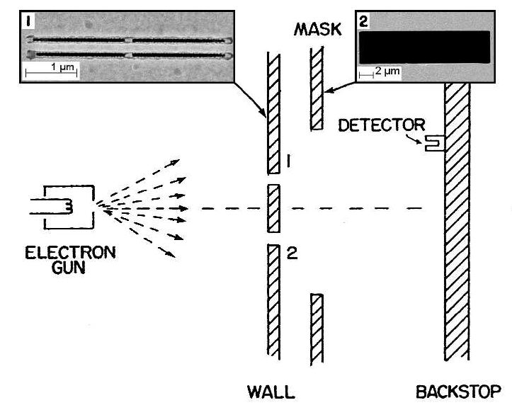
The illustration below relates the actual experimental set-up of a double-slit experiment performed in 2012 to Feynman’s 1965 thought experiment. Indeed, in 1965, the nanotechnology you need for this kind of experiment was not yet available, although the phenomenon of electron diffraction had been confirmed experimentally already in 1925 in the famous Davisson-Germer experiment. [It’s famous not only because electron diffraction was a weird thing to contemplate at the time but also because it confirmed the de Broglie hypothesis only two years after Louis de Broglie had advanced it!]. But so here is the experiment which Feynman thought would never be possible because of technology constraints:
 The insert in the upper-left corner shows the two slits: they are each 50 nanometer wide (50×10–9 m) and 4 micrometer tall (4×10⁻⁶ m). [The thing in the middle of the slits is just a little support. Please do take a few seconds to contemplate the technology behind this feat: 50 nm is 50 millionths of a millimeter. Try to imagine dividing one millimeter in ten, and then one of these tenths in ten again, and again, and once again, again, and again. You just can’t imagine that, because our mind is used to addition/subtraction and – to some extent – with multiplication/division: our mind can’t deal with with exponentiation really – because it’s not a everyday phenomenon.] The second inset (in the upper-right corner) shows the mask that can be moved to close one or both slits partially or completely.
Now, 50 nanometer is 150 times larger than the 0.33 nanometer range we got for ‘our’ electron, but it’s small enough to show diffraction and/or interference. [In fact, in this experiment (done by Bach, Pope, Liou and Batelaan from the University of Nebraska-Lincoln less than two years ago indeed), the beam consisted of electrons with an (average) energy of 600 eV and a de Broglie wavelength of 50 picometer. So that’s like the electrons used in electron microscopes. 50 pm is 6.6 times smaller than the 0.33 nm wavelength we calculated for our low-energy (70 eV) electron – but then the energy and the fact these electrons are guided in electromagnetic fields explain the difference. Let’s go to the results.
The illustration below shows the predicted pattern next to the observed pattern for the two scenarios:
- We first close slit 2, let a lot of electrons go through it, and so we get a pattern described by the probability density function P1 = │Φ1│2. Here we see no interference but a typical diffraction pattern: the intensity follows a more or less normal (i.e. Gaussian) distribution. We then close slit 1 (and open slit 2 again), again let a lot of electrons through, and get a pattern described by the probability density function P2 = │Φ2│2. So that’s how we get P1 and P2.
- We then open both slits, let a whole electrons through, and get according to the pattern described by probability density function P12 = │Φ1+Φ2│2, which we get not from adding the probabilities P1 and P2 (hence, P12 ≠ P1 + P2) – as one would expect if electrons would behave like particles – but from adding the probability amplitudes. We have interference, rather than diffraction.
 But so what exactly is interfering? Well… The electrons. But that can’t be, can it?
The electrons are obviously particles, as evidenced from the impact they make – one by one – as they hit the screen as shown below. [If you want to know what screen, let me quote the researchers: “The resulting patterns were magnified by an electrostatic quadrupole lens and imaged on a two-dimensional microchannel plate and phosphorus screen, then recorded with a charge-coupled device camera. […] To study the build-up of the diffraction pattern, each electron was localized using a “blob” detection scheme: each detection was replaced by a blob, whose size represents the error in the localization of the detection scheme. The blobs were compiled together to form the electron diffraction patterns.” So there you go.]
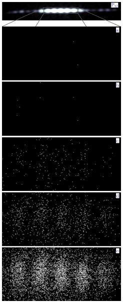
Look carefully at how this interference pattern becomes ‘reality’ as the electrons hit the screen one by one. And then say it: WAW !
Indeed, as predicted by Feynman (and any other physics professor at the time), even if the electrons go through the slits one by one, they will interfere – with themselves so to speak. [In case you wonder if these electrons really went through one by one, let me quote the researchers once again: “The electron source’s intensity was reduced so that the electron detection rate in the pattern was about 1 Hz. At this rate and kinetic energy, the average distance between consecutive electrons was 2.3 × 10⁶ meters. This ensures that only one electron is present in the 1 meter long system at any one time, thus eliminating electron-electron interactions.” You don’t need to be a scientist or engineer to understand that, isn’t it?]
While this is very spooky, I have not seen any better way to describe the reality of the de Broglie wave: the particle is not some point-like thing but a matter wave, as evidenced from the fact that it does interfere with itself when forced to move through two slits – or through one slit, as evidenced by the diffraction patterns built up in this experiment when closing one of the two slits: the electrons went through one by one as well!
But so how does it relate to the characteristics of that wave packet which I described in my previous post? Let me sum up the salient conclusions from that discussion:
- The wavelength λ of a wave packet is calculated directly from the momentum by using de Broglie‘s second relation: λ = h/p. In this case, the wavelength of the electrons averaged 50 picometer. That’s relatively small as compared to the width of the slit (50 nm) – a thousand times smaller actually! – but, as evidenced by the experiment, it’s small enough to show the ‘reality’ of the de Broglie wave.
- From a math point (but, of course, Nature does not care about our math), we can decompose the wave packet in a finite or infinite number of component waves. Such decomposition is referred to, in the first case (finite number of composite waves or discrete calculus) as a Fourier analysis, or, in the second case, as a Fourier transform. A Fourier transform maps our (continuous) wave function, Ψ(x), to a (continuous) wave function in the momentum space, which we noted as φ(p). [In fact, we noted it as Φ(p) but I don’t want to create confusion with the Φ symbol used in the experiment, which is actually the wave function in space, so Ψ(x) is Φ(x) in the experiment – if you know what I mean.] The point to note is that uncertainty about momentum is related to uncertainty about position. In this case, we’ll have pretty standard electrons (so not much variation in momentum), and so the location of the wave packet in space should be fairly precise as well.
- The group velocity of the wave packet (vg) – i.e. the envelope in which our Ψ wave oscillates – equals the speed of our electron (v), but the phase velocity (i.e. the speed of our Ψ wave itself) is superluminal: we showed it’s equal to (vp) = E/p = c2/v = c/β, with β = v/c, so that’s the ratio of the speed of our electron and the speed of light. Hence, the phase velocity will always be superluminal but will approach c as the speed of our particle approaches c. For slow-moving particles, we get astonishing values for the phase velocity, like more than a hundred times the speed of light for the electron we looked at in our previous post. That’s weird but it does not contradict relativity: if it helps, one can think of the wave packet as a modulation of an incredibly fast-moving ‘carrier wave’.
Is any of this relevant? Does it help you to imagine what the electron actually is? Or what that matter wave actually is? Probably not. You will still wonder: How does it look like? What is it in reality?
That’s hard to say. If the experiment above does not convey any ‘reality’ according to you, then perhaps the illustration below will help. It’s one I have used in another post too (An Easy Piece: Introducing Quantum Mechanics and the Wave Function). I took it from Wikipedia, and it represents “the (likely) space in which a single electron on the 5d atomic orbital of an atom would be found.” The solid body shows the places where the electron’s probability density (so that’s the squared modulus of the probability amplitude) is above a certain value – so it’s basically the area where the likelihood of finding the electron is higher than elsewhere. The hue on the colored surface shows the complex phase of the wave function.

So… Does this help?
You will wonder why the shape is so complicated (but it’s beautiful, isn’t it?) but that has to do with quantum-mechanical calculations involving quantum-mechanical quantities such as spin and other machinery which I don’t master (yet). I think there’s always a bit of a gap between ‘first principles’ in physics and the ‘model’ of a real-life situation (like a real-life electron in this case), but it’s surely the case in quantum mechanics! That being said, when looking at the illustration above, you should be aware of the fact that you are actually looking at a 3D representation of the wave function of an electron in orbit.
Indeed, wave functions of electrons in orbit are somewhat less random than – let’s say – the wave function of one of those baryon resonances I mentioned above. As mentioned in my Not So Easy Piece, in which I introduced the Schrödinger equation (i.e. one of my previous posts), they are solutions of a second-order partial differential equation – known as the Schrödinger wave equation indeed – which basically incorporates one key condition: these solutions – which are (atomic or molecular) ‘orbitals’ indeed – have to correspond to so-called stationary states or standing waves. Now what’s the ‘reality’ of that?
The illustration below comes from Wikipedia once again (Wikipedia is an incredible resource for autodidacts like me indeed) and so you can check the article (on stationary states) for more details if needed. Let me just summarize the basics:
- A stationary state is called stationary because the system remains in the same ‘state’ independent of time. That does not mean the wave function is stationary. On the contrary, the wave function changes as function of both time and space – Ψ = Ψ(x, t) remember? – but it represents a so-called standing wave.
- Each of these possible states corresponds to an energy state, which is given through the de Broglie relation: E = hf. So the energy of the state is proportional to the oscillation frequency of the (standing) wave, and Planck’s constant is the factor of proportionality. From a formal point of view, that’s actually the one and only condition we impose on the ‘system’, and so it immediately yields the so-called time-independent Schrödinger equation, which I briefly explained in the above-mentioned Not So Easy Piece (but I will not write it down here because it would only confuse you even more). Just look at these so-called harmonic oscillators below:
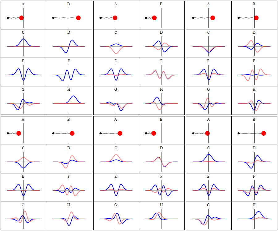
A and B represent a harmonic oscillator in classical mechanics: a ball with some mass m (mass is a measure for inertia, remember?) on a spring oscillating back and forth. In case you’d wonder what the difference is between the two: both the amplitude as well as the frequency of the movement are different. 🙂 A spring and a ball?
It represents a simple system. A harmonic oscillation is basically a resonance phenomenon: springs, electric circuits,… anything that swings, moves or oscillates (including large-scale things such as bridges and what have you – in his 1965 Lectures (Vol. I-23), Feynman even discusses resonance phenomena in the atmosphere in his Lectures) has some natural frequency ω0, also referred to as the resonance frequency, at which it oscillates naturally indeed: that means it requires (relatively) little energy to keep it going. How much energy it takes exactly to keep them going depends on the frictional forces involved: because the springs in A and B keep going, there’s obviously no friction involved at all. [In physics, we say there is no damping.] However, both springs do have a different k (that’s the key characteristic of a spring in Hooke’s Law, which describes how springs work), and the mass m of the ball might be different as well. Now, one can show that the period of this ‘natural’ movement will be equal to t0 = 2π/ω0 = 2π(m/k)1/2 or that ω0 = (m/k)–1/2. So we’ve got a A and a B situation which differ in k and m. Let’s go to the so-called quantum oscillator, illustrations C to H.
C to H in the illustration are six possible solutions to the Schrödinger Equation for this situation. The horizontal axis is position (and so time is the variable) – but we could switch the two independent variables easily: as I said a number of times already, time and space are interchangeable in the argument representing the phase (θ) of a wave provided we use the right units (e.g. light-seconds for distance and seconds for time): θ = ωt – kx. Apart from the nice animation, the other great thing about these illustrations – and the main difference with resonance frequencies in the classical world – is that they show both the real part (blue) as well as the imaginary part (red) of the wave function as a function of space (fixed in the x axis) and time (the animation).
Is this ‘real’ enough? If it isn’t, I know of no way to make it any more ‘real’. Indeed, that’s key to understanding the nature of matter waves: we have to come to terms with the idea that these strange fluctuating mathematical quantities actually represent something. What? Well… The spooky thing that leads to the above-mentioned experimental results: electron diffraction and interference.
Let’s explore this quantum oscillator some more. Another key difference between natural frequencies in atomic physics (so the atomic scale) and resonance phenomena in ‘the big world’ is that there is more than one possibility: each of the six possible states above corresponds to a solution and an energy state indeed, which is given through the de Broglie relation: E = hf. However, in order to be fully complete, I have to mention that, while G and H are also solutions to the wave equation, they are actually not stationary states. The illustration below – which I took from the same Wikipedia article on stationary states – shows why. For stationary states, all observable properties of the state (such as the probability that the particle is at location x) are constant. For non-stationary states, the probabilities themselves fluctuate as a function of time (and space of obviously), so the observable properties of the system are not constant. These solutions are solutions to the time-dependent Schrödinger equation and, hence, they are, obviously, time-dependent solutions.
 We can find these time-dependent solutions by superimposing two stationary states, so we have a new wave function ΨN which is the sum of two others: ΨN = Ψ1 + Ψ2. [If you include the normalization factor (as you should to make sure all probabilities add up to 1), it’s actually ΨN = (2–1/2)(Ψ1 + Ψ2).] So G and H above still represent a state of a quantum harmonic oscillator (with a specific energy level proportional to h), but so they are not standing waves.
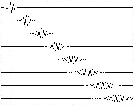
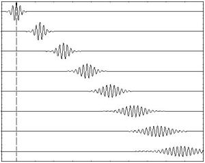
Let’s go back to our electron traveling in a more or less straight path. What’s the shape of the solution for that one? It could be anything. Well… Almost anything. As said, the only condition we can impose is that the envelope of the wave packet – its ‘general’ shape so to say – should not change. That because we should not have dispersion – as illustrated below. [Note that this illustration only represent the real or the imaginary part – not both – but you get the idea.]
That being said, if we exclude dispersion (because a real-life electron traveling in a straight line doesn’t just disappear – as do dispersive wave packets), then, inside of that envelope, the weirdest things are possible – in theory that is. Indeed, Nature does not care much about our Fourier transforms. So the example below, which shows a theoretical wave packet (again, the real or imaginary part only) based on some theoretical distribution of the wave numbers of the (infinite number) of component waves that make up the wave packet, may or may not represent our real-life electron. However, if our electron has any resemblance to real-life, then I would expect it to not be as well-behaved as the theoretical one that’s shown below.

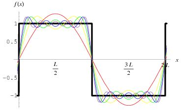
The shape above is usually referred to as a Gaussian wave packet, because of the nice normal (Gaussian) probability density functions that are associated with it. But we can also imagine a ‘square’ wave packet: a somewhat weird shape but – in terms of the math involved – as consistent as the smooth Gaussian wave packet, in the sense that we can demonstrate that the wave packet is made up of an infinite number of waves with an angular frequency ω that is linearly related to their wave number k, so the dispersion relation is ω = ak + b. [Remember we need to impose that condition to ensure that our wave packet will not dissipate (or disperse or disappear – whatever term you prefer.] That’s shown below: a Fourier analysis of a square wave.
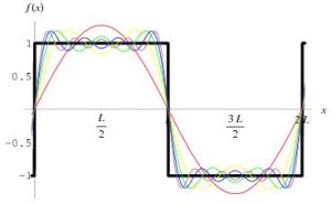
While we can construct many theoretical shapes of wave packets that respect the ‘no dispersion!’ condition, we cannot know which one will actually represent that electron we’re trying to visualize. Worse, if push comes to shove, we don’t know if these matter waves (so these wave packets) actually consist of component waves (or time-independent stationary states or whatever).
[…] OK. Let me finally admit it: while I am trying to explain you the ‘reality’ of these matter waves, we actually don’t know how real these matter waves actually are. We cannot ‘see’ or ‘touch’ them indeed. All that we know is that (i) assuming their existence, and (ii) assuming these matter waves are more or less well-behaved (e.g. that actual particles will be represented by a composite wave characterized by a linear dispersion relation between the angular frequencies and the wave numbers of its (theoretical) component waves) allows us to do all that arithmetic with these (complex-valued) probability amplitudes. More importantly, all that arithmetic with these complex numbers actually yields (real-valued) probabilities that are consistent with the probabilities we obtain through repeated experiments. So that’s what’s real and ‘not so real’ I’d say.
Indeed, the bottom-line is that we do not know what goes on inside that envelope. Worse, according to the commonly accepted Copenhagen interpretation of the Uncertainty Principle (and tons of experiments have been done to try to overthrow that interpretation – all to no avail), we never will.
Some content on this page was disabled on June 20, 2020 as a result of a DMCA takedown notice from Michael A. Gottlieb, Rudolf Pfeiffer, and The California Institute of Technology. You can learn more about the DMCA here:
https://wordpress.com/support/copyright-and-the-dmca/
Some content on this page was disabled on June 20, 2020 as a result of a DMCA takedown notice from Michael A. Gottlieb, Rudolf Pfeiffer, and The California Institute of Technology. You can learn more about the DMCA here:
https://wordpress.com/support/copyright-and-the-dmca/


 We know this elementary wavefunction cannot represent a real-life particle. Indeed, the a·e−i·θ function implies the probability of finding the particle – an electron, a photon, or whatever – would be equal to P(x, t) = |ψ(x, t)|2 = |a·e−(i/ħ)·(E·t−p·x)|2 = |a|2·|e−(i/ħ)·(E·t−p·x)|2 = |a|2·12= a2 everywhere. Hence, the particle would be everywhere – and, therefore, nowhere really. We need to localize the wave – or build a wave packet. We can do so by introducing uncertainty: we then add a potentially infinite number of these elementary wavefunctions with slightly different values for E and p, and various amplitudes a. Each of these amplitudes will then reflect the contribution to the composite wave, which – in three-dimensional space – we can write as:
 Hence, if we don’t change the direction of the y– and z-axes – so we keep defining the z-axis as the axis pointing upwards, and the y-axis as the axis pointing towards us – then the positive direction of the x-axis would actually be the direction from right to left, and we should say that the elementary wavefunction in the animation above seems to propagate in the negative x-direction. [Note that this left- or right-hand rule is quite astonishing: simply swapping the direction of one axis of a left-handed frame makes it right-handed, and vice versa.]

 The next illustration – of how water waves actually propagate – is, perhaps, more relevant. Just think of a two-dimensional equivalent – and of the two oscillations as being transverse waves, as opposed to longitudinal. See how string theory starts making sense? 🙂
 The most fundamental question remains the same: what is it, exactly, that is oscillating here? What is the field? It’s always some force on some charge – but what charge, exactly? Mass? What is it? Well… I don’t have the answer to that. It’s the same as asking: what is electric charge, really? So the question is: what’s the reality of mass, of electric charge, or whatever other charge that causes a force to act on it?
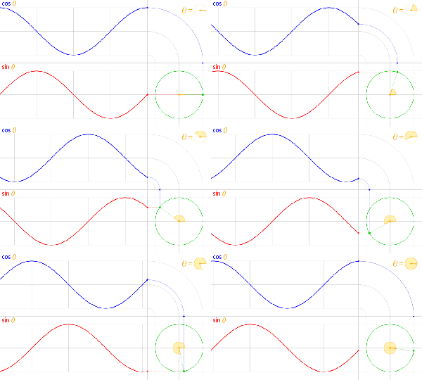 When analyzing this animation – look at the movement of the green, red and blue dots respectively – one cannot miss the equivalence between this oscillation and the movement of a mass on a spring – as depicted below.
 The e−i·(E/ħ)·t function just gives us two springs for the price of one. 🙂 Now, you may want to imagine some kind of elastic medium –