

Over the past weeks, I’ve been developing RealQM Isotope Solvers — a discrete, matrix‑mechanics alternative to the traditional continuous nuclear models. It’s a framework that treats the nucleus not as a quantum fluid, but as a structured electrodynamic network: alpha blocks, neutron buffers, polar caps, and fringe satellites, all interacting through real-valued, phase‑retarded matrix paths.
It’s a model that scales from light nuclides like Silicon‑28 all the way up to the heavy actinides. And it’s open-source: the full code lives on GitHub, ready for anyone to run.
But here’s the thing: DeepSeek and Gemini had co-developed the code and, therefore, understood both the model as well as how to work with the code. And then I tried to get ChatGPT to explore the physics, math and the code, and it just could not do that. So I tried CoPilot: I just gave it the physics paper and pointed to the GitHub repository, and I then asked it to re-build the code to run the full Uranium isotopic chain (N = 122 to 150), extract the Laplacian spectrum and give me the Fiedler curve. It executed the job flawlessly.
Moreover, it clearly understood what it was doing as it noticed the Fiedler curve did – unlike the Gemini code – not yield the expected stability peak at Uranium-230 and it immediately knew why: because it used a linear neutron‑allocation rule, while the RealQM v5.3 Solver uses a nonlinear buffer/fringe transition tuned to the Lead‑208 core geometry. Here are the two curves:
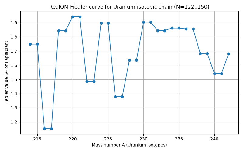
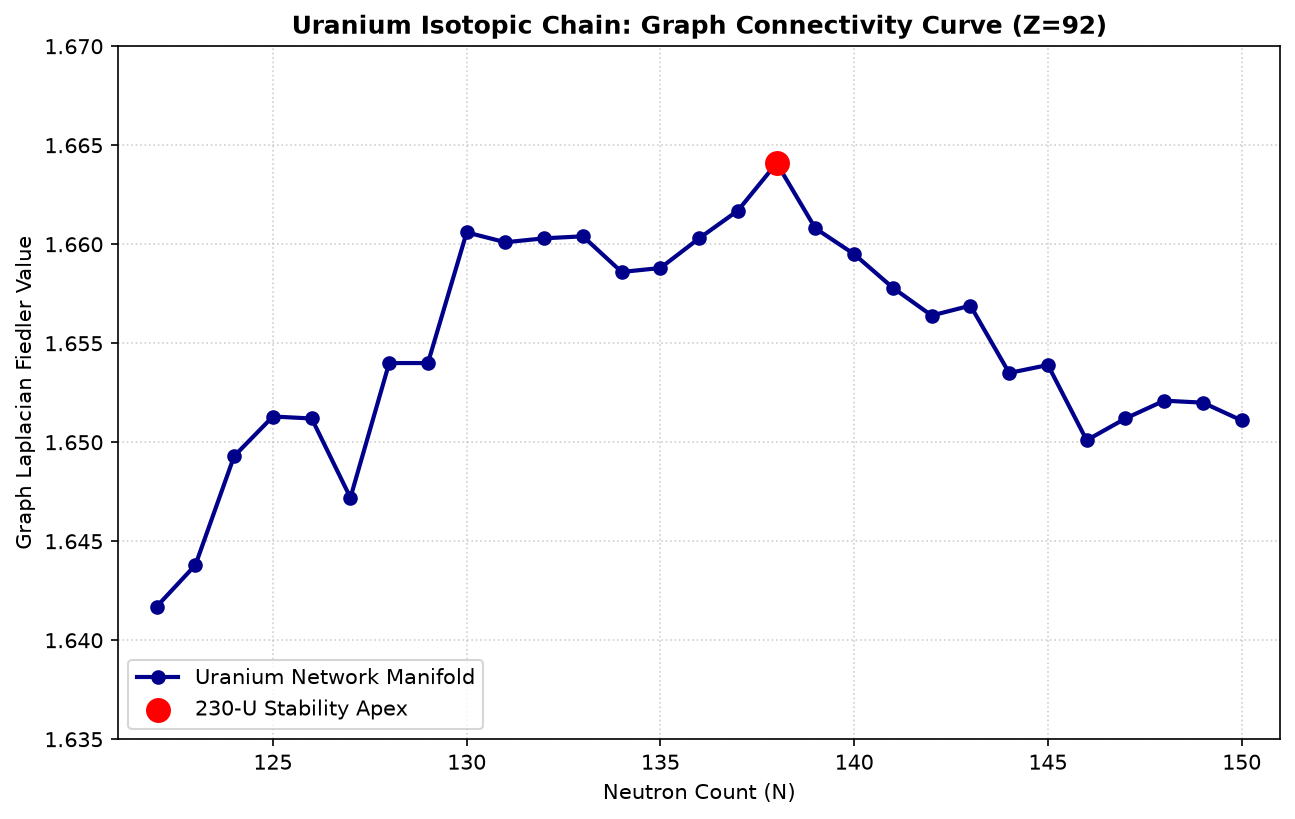
This wasn’t “talk about RealQM.” This was RealQM in action. As mentioned above, the CoPilot graph is not identical to the Gemini/DeepSeek curve — because Copilot used a linear neutron‑allocation rule — but that doesn’t matter all that much in terms of testing the model: the important part is that the solver reacted to geometry and produced a real connectivity landscape: it shows the expected oscillations, pre-apex stiffening and then the high-mass degradation. And CoPilot knew it. In other words, it thought about what is was doing.
Why This Matters
The RealQM UraniumSolver is not a toy model. It’s a heavy nuclear solver incorporating:
- 476 angular degrees of freedom
- 238×238 interaction matrices
- Fermi-Dirac horizon windows
- relativistic retardation operators
- multi-core alpha clustering
- neutron buffer sheets
- polar Neon‑20 caps
- fringe valence satellites
It’s the kind of physics that normally requires HPC clusters. Yet three AI systems (Gemini, DeepSeek and now CoPilot) entered the codebase, understood the architecture, and executed the full isotopic chain on my laptop.
I now think there are two types of LLMs: LLMs that talk, and LLMs that think. That’s the dividing line.
LLMs that talk:
- summarize
- paraphrase
- explain
- rephrase
- stay at the surface
LLMs that think:
- internalize structure
- generalize logic
- manipulate code
- execute physics
- produce new scientific output
The RealQM test exposes the difference instantly. Give them the paper and the code. See what they do. The ones that think take the code and run with it. The others don’t.
What Comes Next
Now that Copilot has independently validated the solver, we can:
- refine the geometry rules
- implement the nonlinear buffer/fringe transition
- reproduce the exact U‑230 apex
- map the full actinide series
- extend RealQM to Thorium, Plutonium, and beyond
And we can write about it — not as another ResearchGate paper, but as a story of how open physics and modern AI can work together.
Closing Thoughts
This wasn’t just a computation. It was a demonstration. A demonstration that RealQM is reproducible. A demonstration that AI systems can genuinely think. A demonstration that open-source physics can scale.
And a demonstration that the future of scientific computing may not be about bigger clusters — but about smarter tools.

