Pre-scriptum (dated 26 June 2020): This post did not suffer from the DMCA take-down of some material. It is, therefore, still quite readable—even if my views on the nature of the Uncertainty Principle have evolved quite a bit as part of my realist interpretation of QM.

Original post:

In previous posts, I presented a time-independent wave function for a particle (or wavicle as we should call it – but so that’s not the convention in physics) – let’s say an electron – traveling through space without any external forces (or force fields) acting upon it. So it’s just going in some random direction with some random velocity v and, hence, its momentum is p = mv. Let me be specific – so I’ll work with some numbers here – because I want to introduce some issues related to units for measurement.

So the momentum of this electron is the product of its mass m (about 9.1×10⁻²⁸ grams) with its velocity v (typically something in the range around 2,200 km/s, which is fast but not even close to the speed of light – and, hence, we don’t need to worry about relativistic effects on its mass here). Hence, the momentum p of this electron would be some 20×10⁻²⁵ kg·m/s. Huh? Kg·m/s?Well… Yes, kg·m/s or N·s are the usual measures of momentum in classical mechanics: its dimension is [mass][length]/[time] indeed. However, you know that, in atomic physics, we don’t want to work with these enormous units (because we then always have to add these ×10⁻²⁸ and ×10⁻²⁵ factors and so that’s a bit of a nuisance indeed). So the momentum p will usually be measured in eV/c, with c representing what it usually represents, i.e. the speed of light. Huh? What’s this strange unit? Electronvolts divided by c? Well… We know that eV is an appropriate unit for measuring energy in atomic physics: we can express eV in Joule and vice versa: 1 eV = 1.6×10⁻¹⁹ Joule, so that’s OK – except for the fact that this Joule is a monstrously large unit at the atomic scale indeed, and so that’s why we prefer electronvolt. But the Joule is a shorthand unit for kg·m²/s², which is the measure for energy expressed in SI units, so there we are: while the SI dimension for energy is actually [mass][length]²/[time]², using electronvolts (eV) is fine. Now, just divide the SI dimension for energy, i.e. [mass][length]²/[time]², by the SI dimension for velocity, i.e. [length]/[time]: we get something expressed in [mass][length]/[time]. So that’s the SI dimension for momentum indeed! In other words, dividing some quantity expressed in some measure for energy (be it Joules or electronvolts or erg or calories or coulomb-volts or BTUs or whatever – there’s quite a lot of ways to measure energy indeed!) by the speed of light (c) will result in some quantity with the right dimensions indeed. So don’t worry about it. Now, 1 eV/c is equivalent to 5.344×10⁻²⁸ kg·m/s, so the momentum of this electron will be 3.75 eV/c.

Let’s go back to the main story now. Just note that the momentum of this electron that we are looking at is a very tiny amount – as we would expect of course.

Time-independent means that we keep the time variable (t) in the wave function Ψ(x, t) fixed and so we only look at how Ψ(x, t) varies in space, with x as the (real) space variable representing position. So we have a simplified wave function Ψ(x) here: we can always put the time variable back in when we’re finished with the analysis. By now, it should also be clear that we should distinguish between real-valued wave functions and complex-valued wave functions. Real-valued wave functions represent what Feynman calls “real waves”, like a sound wave, or an oscillating electromagnetic field. Complex-valued wave functions describe probability amplitudes. They are… Well… Feynman actually stops short of saying that they are not real. So what are they?

They are, first and foremost complex numbers, so they have a real and a so-called imaginary part (z = a + ib or, if we use polar coordinates, re^θ = cosθ + isinθ). Now, you may think – and you’re probably right to some extent – that the distinction between ‘real’ waves and ‘complex’ waves is, perhaps, less of a dichotomy than popular writers – like me 🙂 – suggest. When describing electromagnetic waves, for example, we need to keep track of both the electric field vector E as well as the magnetic field vector B (both are obviously related through Maxwell’s equations). So we have two components as well, so to say, and each of these components has three dimensions in space, and we’ll use the same mathematical tools to describe them (so we will also represent them using complex numbers). That being said, these probability amplitudes,  usually denoted by Ψ(x), describe something very different. What exactly? Well… By now, it should be clear that that is actually hard to explain: the best thing we can do is to work with them, so they start feeling familiar. The main thing to remember is that we need to square their modulus (or magnitude or absolute value if you find these terms more comprehensible) to get a probability (P). For example, the expression below gives the probability of finding a particle – our electron for example – in in the (space) interval [a, b]:

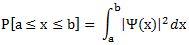
Of course, we should not be talking intervals but three-dimensional regions in space. However, we’ll keep it simple: just remember that the analysis should be extended to three (space) dimensions (and, of course, include the time dimension as well) when we’re finished (to do that, we’d use so-called four-vectors – another wonderful mathematical invention).

Now, we also used a simple functional form for this wave function, as an example: Ψ(x) could be proportional, we said, to some idealized function e^ikx. So we can write: Ψ(x) ∝ e^ikx (∝ is the standard symbol expressing proportionality). In this function, we have a wave number k, which is like the frequency in space of the wave (but then measured in radians because the phase of the wave function has to be expressed in radians). In fact, we actually wrote Ψ(x, t) = (1/x)e^{i(kx – ωt)} (so the magnitude of this amplitude decreases with distance) but, again, let’s keep it simple for the moment: even with this very simple function e^ikx , things will become complex enough.

We also introduced the de Broglie relation, which gives this wave number k as a function of the momentum p of the particle: k = p/ħ, with ħ the (reduced) Planck constant, i.e. a very tiny number in the neighborhood of 6.582 ×10⁻¹⁶ eV·s. So, using the numbers above, we’d have a value for k equal to 3.75 eV/c divided by 6.582 ×10⁻¹⁶ eV·s. So that’s 0.57×10¹⁶ (radians) per… Hey, how do we do it with the units here? We get an incredibly huge number here (57 with 14 zeroes after it) per second? We should get some number per meter because k is expressed in radians per unit distance, right? Right. We forgot c. We are actually measuring distance here, but in light-seconds instead of meter: k is 0.57×10¹⁶/c·s. Indeed, a light-second is the distance traveled by light in one second, so that’s c·s, and if we want k expressed in radians per meter, then we need to divide this huge number 0.57×10¹⁶ (in rad) by 2.998×10⁸ ( in (m/s)·s) and so then we get a much more reasonable value for k, and with the right dimension too: to be precise, k is about 19×10⁶ rad/m in this case. That’s still huge: it corresponds with a wavelength of 0.33 nanometer (1 nm = 10^-6 m) but that’s the correct order of magnitude indeed.

[In case you wonder what formula I am using to calculate the wavelength: it’s λ = 2π/k. Note that our electron’s wavelength is more than a thousand times shorter than the wavelength of (visible) light (we humans can see light with wavelengths ranging from 380 to 750 nm) but so that’s what gives the electron its particle-like character! If we would increase their velocity (e.g. by accelerating them in an accelerator, using electromagnetic fields to propel them to speeds closer to c and also to contain them in a beam), then we get hard beta rays. Hard beta rays are surely not as harmful as high-energy electromagnetic rays. X-rays and gamma rays consist of photons with wavelengths ranging from 1 to 100 picometer (1 pm = 10^–12 m) – so that’s another factor of a thousand down – and thick lead shields are needed to stop them: they are the cause of cancer (Marie Curie’s cause of death), and the hard radiation of a nuclear blast will always end up killing more people than the immediate blast effect. In contrast, hard beta rays will cause skin damage (radiation burns) but they won’t go deeper than that.]

Let’s get back to our wave function Ψ(x) ∝ e^ikx. When we introduced it in our previous posts, we said it could not accurately describe a particle because this wave function (Ψ(x) = Ae^ikx) is associated with probabilities |Ψ(x)|² that are the same everywhere. Indeed,  |Ψ(x)|² = |Ae^ikx|² = A². Apart from the fact that these probabilities would add up to infinity (so this mathematical shape is unacceptable anyway), it also implies that we cannot locate our electron somewhere in space. It’s everywhere and that’s the same as saying it’s actually nowhere. So, while we can use this wave function to explain and illustrate a lot of stuff (first and foremost the de Broglie relations), we actually need something different if we would want to describe anything real (which, in the end, is what physicists want to do, right?). We already said in our previous posts: real particles will actually be represented by a wave packet, or a wave train. A wave train can be analyzed as a composite wave consisting of a (potentially infinite) number of component waves. So we write:

Note that we do not have one unique wave number k or – what amounts to saying the same – one unique value p for the momentum: we have n values. So we’re introducing a spread in the wavelength here, as illustrated below:

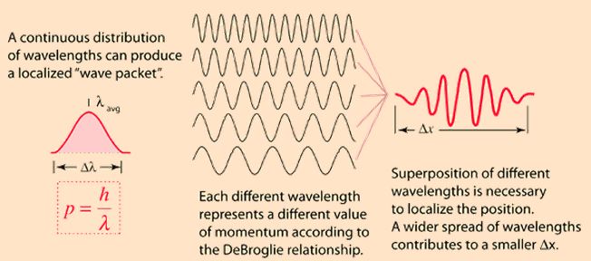
In fact, the illustration above talks of a continuous distribution of wavelengths and so let’s take the continuum limit of the function above indeed and write what we should be writing:

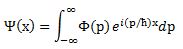
Now that is an interesting formula. [Note that I didn’t care about normalization issues here, so it’s not quite what you’d see in a more rigorous treatment of the matter. I’ll correct that in the Post Scriptum.] Indeed, it shows how we can get the wave function Ψ(x) from some other function Φ(p). We actually encountered that function already, and we referred to it as the wave function in the momentum space. Indeed, Nature does not care much what we measure: whether it’s position (x) or momentum (p), Nature will not share her secrets with us and, hence, the best we can do – according to quantum mechanics – is to find some wave function associating some (complex) probability amplitude with each and every possible (real) value of x or p. What the equation above shows, then, is these wave functions come as a pair: if we have Φ(p), then we can calculate Ψ(x) – and vice versa. Indeed, the particular relation between Ψ(x) and Φ(p) as established above, makes Ψ(x) and Φ(p) a so-called Fourier transform pair, as we can transform Φ(p) into Ψ(x) using the above Fourier transform (that’s how that  integral is called), and vice versa. More in general, a Fourier transform pair can be written as:

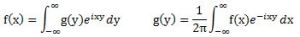
Instead of x and p, and Ψ(x) and Φ(p), we have x and y, and f(x) and g(y), in the formulas above, but so that does not make much of a difference when it comes to the interpretation: x and p (or x and y in the formulas above) are said to be conjugate variables. What it means really is that they are not independent. There are quite a few of such conjugate variables in quantum mechanics such as, for example: (1) time and energy (and time and frequency, of course, in light of the de Broglie relation between both), and (2) angular momentum and angular position (or orientation). There are other pairs too but these involve quantum-mechanical variables which I do not understand as yet and, hence, I won’t mention them here. [To be complete, I should also say something about that 1/2π factor, but so that’s just something that pops up when deriving the Fourier transform from the (discrete) Fourier series on which it is based. We can put it in front of either integral, or split that factor across both. Also note the minus sign in the exponent of the inverse transform.]

When you look at the equations above, you may think that f(x) and g(y) must be real-valued functions. Well… No. The Fourier transform can be used for both real-valued as well as complex-valued functions. However, at this point I’ll have to refer those who want to know each and every detail about these Fourier transforms to a course in complex analysis (such as Brown and Churchill’s Complex Variables and Applications (2004) for instance) or, else, to a proper course on real and complex Fourier transforms (they are used in signal processing – a very popular topic in engineering – and so there’s quite a few of those courses around).

The point to note in this post is that we can derive the Uncertainty Principle from the equations above. Indeed, the (complex-valued) functions Ψ(x) and Φ(p) describe (probability) amplitudes, but the (real-valued) functions |Ψ(x)|² and |Φ(p)|² describe probabilities or – to be fully correct – they are probability (density) functions. So it is pretty obvious that, if the functions Ψ(x) and Φ(p) are a Fourier transform pair, then |Ψ(x)|² and |Φ(p)|² must be related to. They are. The derivation is a bit lengthy (and, hence, I will not copy it from the Wikipedia article on the Uncertainty Principle) but one can indeed derive the so-called Kennard formulation of the Uncertainty Principle from the above Fourier transforms. This Kennard formulation does not use this rather vague Δx and Δp symbols but clearly states that the product of the standard deviation from the mean of these two probability density functions can never be smaller than ħ/2:

σ_xσ_p ≥ ħ/2

To be sure: ħ/2 is a rather tiny value, as you should know by now, 🙂 but, so, well… There it is.

As said, it’s a bit lengthy but not that difficult to do that derivation. However, just for once, I think I should try to keep my post somewhat shorter than usual so, to conclude, I’ll just insert one more illustration here (yes, you’ve seen that one before), which should now be very easy to understand: if the wave function Ψ(x) is such that there’s relatively little uncertainty about the position x of our electron, then the uncertainty about its momentum will be huge (see the top graphs). Vice versa (see the bottom graphs), precise information (or a narrow range) on its momentum, implies that its position cannot be known.

Does all this math make it any easier to understand what’s going on? Well… Yes and no, I guess. But then, if even Feynman admits that he himself “does not understand it the way he would like to” (Feynman Lectures, Vol. III, 1-1), who am I? In fact, I should probably not even try to explain it, should I? 🙂

So the best we can do is try to familiarize ourselves with the language used, and so that’s math for all practical purposes. And, then, when everything is said and done, we should probably just contemplate Mario Livio’s question: Is God a mathematician? 🙂

Post scriptum:

I obviously cut corners above, and so you may wonder how that ħ factor can be related to σ_x and σ _p if it doesn’t appear in the wave functions. Truth be told, it does. Because of (i) the presence of ħ in the exponent in our e^i(p/ħ)x function, (ii) normalization issues (remember that probabilities (i.e. Ψ|(x)|² and |Φ(p)|²) have to add up to 1) and, last but not least, (iii) the 1/2π factor involved in Fourier transforms , Ψ(x) and Φ(p) have to be written as follows:

Note that we’ve also re-inserted the time variable here, so it’s pretty complete now. One more thing we could do is to substitute x for a proper three-dimensional space vector x or, better still, introduce four-vectors, which would allow us to also integrate relativistic effects (most notably the slowing of time with motion – as observed from the stationary reference frame) – which become important when, for instance, we’re looking at electrons being accelerated, which is the rule, rather than the exception, in experiments.

Remember (from a previous post) that we calculated that an electron traveling at its usual speed in orbit (2200 km/s, i.e. less than 1% of the speed of light) had an energy of about 70 eV? Well, the Large Electron-Positron Collider (LEP) did accelerate them to speeds close to light, thereby giving them energy levels topping 104.5 billion eV (or 104.5 GeV as it’s written) so they could hit each other with collision energies topping 209 GeV (they come from opposite directions so it’s two times 104.5 GeV). Now, 209 GeV is tiny when converted to everyday energy units: 209 GeV is 33×10^–9 Joule only indeed – and so note the minus sign in the exponent here: we’re talking billionths of a Joule here. Just to put things into perspective: 1 Watt is the energy consumption of an LED (and 1 Watt is 1 Joule per second), so you’d need to combine the energy of billions of these fast-traveling electrons to power just one little LED lamp. But, of course, that’s not the right comparison: 104.5 GeV is more than 200,000 times the electron’s rest mass (0.511 MeV), so that means that – in practical terms – their mass (remember that mass is a measure for inertia) increased by the same factor (204,500 times to be precise). Just to give an idea of the effort that was needed to do this: CERN’s LEP collider was housed in a tunnel with a circumference of 27 km. Was? Yes. The tunnel is still there but it now houses the Large Hadron Collider (LHC) which, as you surely know, is the world’s largest and most powerful particle accelerator: its experiments confirmed the existence of the Higgs particle in 2013, thereby confirming the so-called Standard Model of particle physics. [But I’ll see a few things about that in my next post.]

Oh… And, finally, in case you’d wonder where we get the inequality sign in σ_xσ_p ≥ ħ/2, that’s because – at some point in the derivation – one has to use the Cauchy-Schwarz inequality (aka as the triangle inequality): |z₁+ z₁| ≤ |z₁|+| z₁|. In fact, to be fully complete, the derivation uses the more general formulation of the Cauchy-Schwarz inequality, which also applies to functions as we interpret them as vectors in a function space. But I would end up copying the whole derivation here if I add any more to this – and I said I wouldn’t do that. 🙂 […]