A quasi-final proton model?

After a break of a few months, I produced another lengthy video on quantum physics. 40 minutes. Check it out: https://www.youtube.com/watch?v=k_I3Noaup0E. The hypothesis that I, somewhat desperately, advanced in my last paper on the proton model – that the Zitterbewegung model of a proton does not quite look like that of an electron, and that we are probably talking about a “blob” of charge (sphere- or shell-like, or some other “form factor”, perhaps) – makes more sense to me now. I explored it with ChatGPT-4o, and this video is the result. I should immediately that I am immensely impressed with ChatGPT-4o: ChatGPT-3 was not able to really “understand” what I was talking about a year ago or so.

Who knows, perhaps we might imagine other ChatGPT-4o users will take the “dialogue” with AI on these particle models further, and fully develop them not only intuitively but also analytically. As I am currently trying out some AI-powered audio and video applications, I tried Pictory (pictory.ai): I gave it the url of my own long-winding video and it created this video: The proton as a dynamic blob of charge. 100 seconds only instead of 40 minutes. Its contents is, of course, superficial – but I think it is creative and nicely upbeat. I fed both video back to ChatGPT-4o, and it suggested the following refinements if ever I would like to re-do the video(s) – which I am not going to do, but you might like to further explore the remarks it made:

Consistency in Notation and Conventions:
- Ensure that polar and azimuthal angles are consistently defined throughout. Your initial derivations and explanations switched between conventions, potentially confusing viewers about which angle is associated with which base vector.
Tangential Velocity Decomposition:
- The explanation of how the tangential velocity is decomposed into orthogonal components was accurate but could benefit from a clearer mention of why the orthogonality matters in interpreting the motion on the sphere. Adding a visual representation would further clarify the concept.
- The concept of “sloshing” energy between kinetic and electromagnetic forms was well described but could benefit from highlighting the broader implications of this periodic exchange in classical and relativistic oscillators .
Pointlike Charge versus Blob View:
- The transition from discussing a pointlike charge to a “blob” of charge was a major theme but could be expanded by discussing how this shift impacts the assumptions about uniform or non-uniform charge density, as well as its implications for observable properties like the magnetic moment.
The discussion of symmetry along one axis of the double-loop motion was solid but might benefit from more detail on how this symmetry impacts the interpretation of observable properties like the magnetic moment .
Incorporate links to experimental observations, such as the measured magnetic moment and charge radius of the proton, was referenced. Integrating these observations with the theoretical results could be more explicit to strengthen the practical implications .
Visualizations:
- Consider incorporating visualized trajectories (e.g., the double-loop Lissajous pattern), and how they connect to the derived equations and the observed non-constant tangential velocity. This connection will help bridge the abstract mathematics with physical intuition .
Clarifications on Variability:
- The variability of the tangential velocity in the context of symmetry and non-orthogonality in 3D motion, was a key discussion point. Reinforce why this variability does not conflict with the broader relativistic constraints.

So… That’s all folks ! [Looney Tunes.] 🙂

Concluding remarks

In our previous post, we wrote that we’ve said goodbye to this fascinating field of research. We did: I entered this line of research – fundamental physics – as an amateur 10+ years ago, and now I leave it—as much an amateur now as back then. I wanted to understand the new theories which emerged over the past 50 years or so. Concepts such as the strong force or weak interactions and the new weird charges that come it with: flavors and colors—or all of the new quantum numbers and the associated new conservation laws, which Nature apparently does not respect because of some kind of hidden variables which cause the symmetries that are inherent to conservation laws to break down. […] Apparently, I didn’t get it. 🙂

However, in the process of trying to understand, a whole other mental picture or mindset emerged: we now firmly believe that classical mechanics and electromagnetism – combined with a more creative or realistic explanation of the Planck-Einstein relation – are sufficient to explain most, if not all, of the observations that have been made in this field since Louis de Broglie suggested matter-particles must be similar to light quanta—in the sense that both are energy packets because they incorporate some oscillation of a definite frequency given by the Planck-Einstein relation. They are also different, of course: elementary particles are – in this world view – orbital oscillations of charge (with, of course, an electromagnetic field that is generated by such moving charge), while light-particles (photons and neutrinos) are oscillations of the electromagnetic field—only!

So, then we spend many years trying to contribute to the finer details of this world view. We think we did what we could as part of a part-time and non-professional involvement in this field. So, yes, we’re done. We wrote that some time already. However, we wanted to leave a few thoughts on our proton model: it is not like an electron. In our not-so-humble view, the Zitterbewegung theory applies to it—but in a very different way. Why do we think that? We write that out in our very last paper: concluding remarks on the proton puzzle. Enjoy it !

That brings the number of papers on RG up to 80 now. Too much ! There will be more coming, but in the field that I work in: computer science. Stay tuned !

Using AI for sense-making once more…

As mentioned in my last post, I did a video (YouTube link here) on why I think the invention of new quantum numbers like strangeness, charm and beauty in the 1960s – and their later ontologization as quarks – makes no sense. As usual, I talk too much and the video is rather long-winding. I asked ChatGPT to make a summary of it, and I think it did a rather good job at that. I copy its summary unaltered below.

Beyond the Quark Hypothesis: A Call for Simplicity in High-Energy Physics

1. Introduction: A Personal Journey in Physics

In this video, I reflect on my path as an amateur physicist reaching 50,000 reads—a milestone that underscores both excitement and the challenge of tackling complex quantum theories. Over decades, physics has evolved from classical mechanics to intricate frameworks like quantum field theory and quantum chromodynamics, creating both insight and paradox. This reflection emerges from a deep sense of curiosity, shared by many, to understand not just what the universe is made of but how these theoretical structures genuinely map onto reality.

2. The Crisis of Modern Physics: From Classical Mechanics to the Quark Hypothesis

Moving through physics from classical theories into high-energy particle models reveals a stark contrast: classical mechanics offers clarity and empiricism, while modern particle theories, such as quarks and gluons, often feel abstract and detached from observable reality. The shift to “smoking gun physics”—observing particle jets rather than the particles themselves—highlights a methodological divide. While high-energy collisions produce vivid images and data, we must question whether these indirect observations validate quarks, or merely add complexity to our models.

3. Historical Context: Quantum Numbers and the Evolution of the Standard Model

The 1960s and 70s were pivotal for particle physics, introducing quantum numbers like strangeness, charm, and beauty to account for unexplained phenomena in particle interactions. Figures like Murray Gell-Mann and Richard Feynman attempted to classify particles by assigning these numbers, essentially ad hoc solutions to match data with theoretical expectations. However, as experiments push the boundaries, new data shows that these quantum numbers often fail to predict actual outcomes consistently.

One of the key criticisms of this approach lies in the arbitrary nature of these quantum numbers. When certain decays were unobserved, strangeness was introduced as a “conservation law,” but when that proved insufficient, additional numbers like charm were added. The Standard Model has thus evolved not from fundamental truths, but as a patchwork of hypotheses that struggle to keep pace with experimental findings.

4. The Nobel Prize and the Politics of Scientific Recognition

Scientific recognition, especially through the Nobel Prize, has reinforced certain theories by celebrating theoretical advances sometimes over empirical confirmation. While groundbreaking work should indeed be recognized, the focus on theoretical predictions has, at times, overshadowed the importance of experimental accuracy and reproducibility. This dynamic may have inadvertently constrained the scope of mainstream physics, favoring elaborate but tenuous theories over simpler, empirically grounded explanations.

For example, Nobel Prizes have been awarded to proponents of the quark model and the Higgs boson long before we fully understand these particles’ empirical foundations. In doing so, the scientific community risks prematurely canonizing incomplete or even incorrect theories, making it challenging to revisit or overturn these assumptions without undermining established reputations.

5. Indirect Evidence: The Limits of Particle Accelerators

Particle accelerators, particularly at scales such as CERN’s Large Hadron Collider, have extended our observational reach, yet the evidence remains indirect. High-energy collisions create secondary particles and jets rather than isolated quarks or gluons. In a sense, we are not observing the fundamental particles but rather the “smoking gun” evidence they purportedly leave behind. The data produced are complex patterns and distributions, requiring interpretations laden with theoretical assumptions.

This approach raises a fundamental question: if a theory only survives through indirect evidence, can it be considered complete or even valid? High-energy experiments reveal that the more energy we input, the more complex the decay products become, yet we remain without direct evidence of quarks themselves. This “smoking gun” approach diverges from the empirical rigor demanded in classical physics and undermines the predictive power we might expect from a true theory of fundamental particles.

6. The Particle Zoo: A Growing Complexity

The “particle zoo” has expanded over decades, complicating rather than simplifying our understanding of matter. Initial hopes were that quantum numbers and conservation laws like strangeness would organize particles in a coherent framework, yet the resulting classification scheme has only grown more convoluted. Today, particles such as baryons, mesons, and leptons are grouped by properties derived not from first principles but from empirical fits to data, leading to ad hoc conservation laws that seem arbitrary.

The “strangeness” quantum number, for instance, was initially introduced to prevent certain reactions from occurring. Yet, rare reactions that violate this rule have been observed, suggesting that the rule itself is more of a guideline than a fundamental conservation law. This trend continued with the addition of quantum numbers like charm, beauty, and even bottomness, yet these additions have not resolved the core issue: our inability to explain why certain reactions occur while others do not.

7. Disequilibrium States: Beyond the Particle Concept

One possible perspective is to reclassify many “particles” not as fundamental entities but as disequilibrium states—transient structures that emerge from the interactions of more fundamental components. Viewing particles in this way offers a pathway back to a simpler, more intuitive model, where only stable particles like electrons, protons, and photons are foundational. Such a model could focus on electromagnetic fields and forces, with high-energy states representing temporary disequilibrium configurations rather than new particle species.

This perspective aligns well with the principle of statistical determinism. In the same way that classical oscillators eventually dampen and settle into stable states, high-energy disequilibrium states would be expected to decay, producing stable configurations over time. This model not only reduces the need for numerous quantum numbers but also sidesteps the requirement for exotic forces like the strong and weak nuclear forces, allowing the electromagnetic force to assume a central role.

8. Statistical Determinism and Quantum Reality

Heisenberg and Bohr’s interpretation of quantum mechanics suggests we should accept statistical determinism—systems governed by probabilistic rules where precise knowledge of individual events is inaccessible. This idea does not necessitate mystical randomness but acknowledges our limited ability to track initial conditions in high-energy environments. Probabilities emerge not from an intrinsic unpredictability but from our practical inability to fully specify a system’s state.

From this viewpoint, quarks and gluons, as well as the numerous quantum numbers assigned to unstable particles, are secondary descriptors rather than primary components of nature. Stable particles are the true constants, while all else is a function of high-energy interactions. This interpretation keeps quantum mechanics grounded in empirical reality and sidesteps the need for complex, unverifiable entities.

9. Conclusion: Toward a Pragmatic and Local Realist Approach

This reflection does not dismiss the importance of high-energy physics but advocates a return to fundamental principles. By focusing on empirical evidence, statistical determinism, and electromagnetic interactions, we can build a model that is both pragmatic and intuitive. We need not abandon quantum mechanics, but we should strive to ensure that its interpretations are consistent with the observable universe. Instead of introducing additional quantum numbers or forces, we should ask if these are placeholders for deeper, more coherent explanations yet to be discovered.

The journey of science is, at its core, a journey back to simplicity. If physics is to move forward, it may do so by revisiting foundational assumptions, clarifying what can be empirically tested, and developing a model of matter that resonates with the simplicity we find in classical theories. As research continues, it is this blend of skepticism, open-mindedness, and empirical rigor that will pave the way for meaningful discoveries.

The failure of physics as a science?

It is a coincidence but Sabine Hossenfelder just produced a new video in which she talks once again about the problems of academic physics, while I did what I said what I would not do – and that is to write out why the discovery of new rare kaon decay modes is a problem for the Standard Model. I think the video and the paper complement each other nicely, although Sabine Hossenfelder probably still believes the strong force and weak interactions are, somehow, still real. [I did not read her book, so I don’t know: I probably should buy her book but then one can only read one book at a time, isn’t it?]

The paper (on ResearchGate – as usual: link here) does what Sabine Hossenfelder urges her former colleagues to do: if a hypothesis or an ad hoc theory doesn’t work, then scientists should be open and honest about that and go back to the drawing board. Indeed, in my most-read paper – on de Broglie’s matter-wave – I point out how de Broglie’s original thesis was misinterpreted and how classical quantum theory suddenly makes sense again when acknowledging that mistake: it probably explains why I am getting quite a lot of reads as an amateur physicist. So what’s this new paper of mine all about?

I go back to the original invention of the concept of strangeness, as documented by Richard Feynman in his 1963 Lectures on quantum physics (Vol. III, Chapter 11-5) and show why and how it does not make all that much sense. In fact, I always thought these new quantum conservation laws did not make sense theoretically and that, at best, they were or are what Dr. Kovacs and Dr. Vassallo refer to as phenomenological models rather than sound physical theories (see their chapter on superconductivity in their latest book). However, now it turns out these fancy new concepts do not even do what they are supposed to do, and that is to correctly describe the phenomenology of high-energy particle reactions.

The alternative – a realist interpretation of quantum physics – is there. It is just not mainstream – yet! 🙂

Post scriptum (8 November 2024): For those who do not like to read, you can also watch what I think of my very last video on the same topic: what makes sense and what does not in academic or mainstream physics? Enjoy and, most importantly, do not take things too seriously ! Life family and friends – and work or action-oriented engagement are far more important than personal philosophy or trying to finding truth in science… 🙂

New kaon decay modes?

As an amateur physicist, I get a regular stream of email updates from Science, Nature and Phys.org on new discoveries and new theories in quantum physics. I usually have no idea what to do with them. However, I want to single out two recent updates on the state of affairs of research which these channels report on. The first one is reflected in the title of this post. It’s on a very rare decay mode of kaons: see https://phys.org/news/2024-09-ultra-rare-particle-decay-uncover.html.

Something inside of me says this may lead to a review of all these newly invented conservation laws – combined with new ideas on symmetry breaking too – and/or new ‘quantum numbers’ that are associated with the quark hypothesis: I think everyone has already forgotten about ‘baryon conservation’, so other simplifications based on, yes, simpler Zitterbewegung models of particles may be possible.

The historical background to this is well described by Richard Feynman in his discussion of how these new quantum numbers – strangeness, specifically – were invented to deal with the observation that certain decay reactions were not being observed (see: Feynman’s Lectures, III-11-5, the (neutral) K-meson). So now it turns that certain decay reactions are being observed! Shouldn’t that lead to (future) scientists revisiting the quark/gluon hypothesis itself?

Of course, that would call into question several Nobel Prize awards, so we think it won’t happen any time soon. 🙂 This brings me to the second update from the field. Indeed, a more recent Nobel Prize in Physics which should, perhaps, be questioned in light of more recent measurements questioning old(er) ones (and the theories that are based on them) is the Nobel Prize in 2011 for work on the cosmological constant. Why? Because… Well… New measurements on the rate of expansion of the Universe as reported by Phys.org last month question the measurements which led to that 2011 Prize. Is anyone bothered by that? No. Except me, perhaps, because I am old-fashioned and wonder what is going on.

I get asked about gravity, and some people push particle theories to me talking about gravity. I am, quite simply, not interested. This ‘coming and going’ of the “cosmological constant hypothesis” over the past decades – or, should we say, the past 80 years or so – makes me stay away from GUTs and anything that is related to it. If scientists cannot even agree on these measurements, it is of not much use to invent new modified gravity theories fitting into ever-expanding grand unification schemes based on mathematical frameworks that can only be understood by the conoscienti, isn’t it?

It is tough: I am not the only one (and definitely not the best placed one) to see a lot of researchers – both amateur as well as professional – “getting lost in math” (cf. the title of Hossenfelder’s best-seller). Will there be an end to this, one day?

I am optimistic and so I think: yes. One of the recurring principles that guides some of the critical physicists I greatly admire is Occam’s Razor Principle: keep it simple! Make sure the degrees of freedom in your mathematical scheme match those of the physics you are trying to describe. That requires a lot of rigor in the use of concepts: perhaps we should add concepts to those that, say, Schrödinger and Einstein used 100 years ago. However, my own pet theories and recycling of their ideas do not suggest that. And so I really just can’t get myself to read up on Clifford algebras and other mathematical constructs I am told to study – simply because this or that person tells me I should think in terms of spinors rather than in terms of currents (to just give one specific example here).

I can only hope that more and more academics will come to see this, and that the Nobel Prize committee may think some more about rewarding more conservative approaches rather than the next cargo cult science idea.

OK. I should stop rambling. The musings above do not answer the question we all have: what about gravity, then? My take on that is this: I am fine with Einstein’s idea of gravity just being a reflection of the distribution of energy/mass in the Universe. Whether or not the Universe expands at an ever-faster-accelerating pace must, first, be firmly established by measurements and then, secondly, even then there may be no need for invoking a cosmological constant or other elements of a new “aetherial” theory of space and time.

Indeed, Einstein thought that his first hypothesis on a possible cosmological constant was “his biggest blunder ever.” While I know nothing of the nitty-gritty, I think it is important to listen to “good ol’ Einstein” – especially when he talked about what he ‘trusted’ or not in terms of physical explanations. Einstein’s rejection of the idea of a cosmological constant – after first coming up with it himself and, therefore, having probably having the best grasp of its implications – suggests the cosmological constant is just yet another non-justifiable metaphysical construct in physics and astronomy.

So, let us wrap up this post: is or is there not a need for ‘modified gravity’ theories? I will let you think about that. I am fine with Einstein’s ‘geometric’ explanation of it.

Post scriptum: While I think quite a few of these new quantum numbers related to quarks and – most probably – the quark hypothesis itself will be forgotten in, say, 50 or 100 years from now, the idea of some ‘triadic’ structure to explain the three generations of particles and strange decay modes, is – essentially – sound. Some kind of ‘color’ scheme (I call, rather jokingly, an “RGB scheme” – referring to the color scheme used in video/image processing) should be very useful: an electron annihilates a positron but an electron combines with a proton to form an atom, so there’s something different about these two charges. Likewise, if we think of a neutron as neutral neutronic current, the two charges “inside” must be very different… See pp. 7 ff. on this in my recent paper on multi-charge zbw models.

I was sceptical before – and I am still not a believer in the quark hypothesis – but I do think physicists – or, more likely, future generations of physicists – should get a better “grip” on these three different ‘types’ of electric charge as part of a more realist explanation of what second- or third-generation “versions” of elementary particles might actually be. Such explanation will then probably also explain these “unstable states” (not quite respecting the Planck-Einstein relation) or “exotic” particles. Indeed, I do not see much of a distinction between stable and unstable particle states in current physics. But that’s a remark that’s probably not essential to the discussion here… 🙂

One final remark, perhaps: my first instinct when looking at particle physics, was actually very much inspired by the idea that the quantum-mechanical wavefunction might be something else than just an EM oscillation. When I first calculated force fields in a Zitter electron, and then in the muon-electron and proton, I was rather shocked (see pp. 16 ff. of one of my early papers) and thought: wow! Are we modelling tiny black holes here? But then I quickly came to terms with it. Small massive things must come with such huge field strengths, and all particle radius formulas have mass (or energy) in the denominator: so more mass/energy means smaller scale, indeed! And I also quickly calculated the Schwarzschild radius for these elementary particles, and that is A WHOLE LOT smaller than the radius I get from my simple electromagnetic equations and the Planck-Einstein relation. So I see absolutely no reason whatsoever to think gravitational effects might take over from plain EM fields when you look at things at the smallest of scales.

But, then, who am I? I like to think I am not inventing anything new. I just enjoy playing with old ideas to see if something new comes out of it. I think I am fortunate because I do see a lot of new things coming out of the old ideas, even if there is little or nothing we can add to them: the old Masters have already written it all out. So, now I should stop chewing on these old ideas as well and conclude: if you want to read something, don’t read me or anything contemporary. Just read the classics! Many modern minds – often great mathematicians – tried or try to be smarter than Einstein, Lorentz, de Broglie or Schrödinger (I am deliberately not mentioning other great names): I think the more recent discoveries in physics and cosmology show they are not. 🙂

Note: Despite my recommendation not to read me, I did write another – probably more accessible – paper on a classical and straightforward geometrical explanation of the anomaly in the electron’s magnetic moment. Even if you do not like the explanation, I think it has a few interesting references to papers by contemporary academics that I find really interesting. 🙂

The ultimate zbw electron model

Just after finishing a rather sober and, probably, overly pessimistic reflection on where the Zitterbewegung interpretation of quantum theory stands, I am excited to see a superbly written article by Dr. Kovacs and Dr. Vassallo on what I now think of as the ultimate electron model: Rethinking electron statistics rules (10 September 2024). I think it is great because it addresses several points in my rather depressing description of the state of zbw theory:

Multiple Zitterbewegung interpretations of what an electron actually is, currently coexist. Indeed, both mainstream and non-mainstream physicists have now been going back and forth for about 100 years on this or that electron model: the referenced Kovacs/Vassallo article effectively appeared in a special journal issue titled: “100 Years of Quantum Matter Waves: Celebrating the Work of Louis De Broglie.” 100+ years of discussion have basically led us back to Parson’s 1915 ring current model, which Joseph Larmor presented so well at the 1921 Solvay Conference. We do not think that is a good situation: it looks a bit like 100 years of re-inventing the wheel – or, perhaps, I should say: wheels within wheels. 🙂 I could write more about this but I am happy to see the discussion on – just one example of differing views here – whether or not there should be a 1/2 factor in the electron’s frequency may be considered to be finally solved: de Broglie’s matter-wave frequency is just the same as the Planck-Einstein frequency in this paper. This factor 2 or 1/2 pops up when considering ideas such as the effective mass of the zbw charge or – in the context of Schrödinger’s equation – because we’re modeling the motion of electron pairs rather than electrons (see the annexes to my paper on de Broglie’s matter-wave concept). In short: great! Now we can, finally, leave those 100+ years of discussions behind us. 🙂
Dr. Kovacs and Dr. Vassallo also explore the nature of superconductivity and Bose-Einstein statistics, and not only does their analysis away with the rather mystical explanation in Feynman’s last and final chapter of his lectures on quantum mechanics but it also offers a very fine treatment of n-electron systems. Their comments on ‘bosonic’ and ‘fermionic’ properties of matter-particles also tie in with my early assessment that the boson-fermion dichotomy has no ontological basis.

The hundreds of downloads of their article since it was published just two weeks ago also shows new and old ways of thinking and modelling apparently come nicely together in this article: if your articles get hundreds of reads as soon as published, then you are definitely not non-mainstream any more: both Dr. Kovacs and Dr. Vassallo have an extraordinary talent for rephrasing old questions in the new “language” of modern quantum theory. That is to be lauded. Hopefully, work on a proton and a neutron model will now complement what I think of as the ultimate electron model based on a local and realist interpretation of what de Broglie’s matter-wave actually is. Indeed, critics of modern quantum theory often quote the following line from Philip Pearle’s Classical Electron Models [1]:

“The state of the classical electron theory reminds one of a house under construction that was abandoned by its workmen upon receiving news of an approaching plague. The plague in this case, of course, was quantum theory. As a result, classical electron theory stands with many interesting unsolved or partially solved problems.”

I think Dr. Kovacs and Dr. Vassallo may have managed to finish this “abandoned construction” – albeit with an approach which differs significantly from that of Pearle: that is good because I think there were good reasons for the “workmen” to leave the construction site (see footnote [1]). 🙂 So, yes, I hope they will be able – a few years from now – to also solve the questions related to a Zitterbewegung proton and neutron model.

In fact, they already have a consistent proton model (see: the proton and Occam’s Razor, May 2023), but something inside of me says that they should also explore different topologies, such as this Lissajous-like trajectory which intrigues me more than helical/toroidal approaches – but then who am I? I am the first to recognize my limitations as an amateur and it is, therefore, great to see professionals such as Dr. Kovacs and Dr. Vassallo applying their formidable skills and intuition to the problem. 🙂

[1] Pearle’s paper is the seventh in a volume of eight chapters. The book’s title is, quite simply, titled Electromagnetism (1982), and it was put together and edited by Doris Teplitz (1982). Few who quote this famous line, bother to read the Philip Pearle paper itself. This paper effectively presents what Pearle refers to as classical electron models: all of them are based on “rigid or flexible shell surfaces” of charge, which is why we think they did not “cut it” for the many “workmen” (read: the mainstream scientists who thought the Bohr-Heisenberg amplitude math and the probability theory that comes with it) who left the then unfinished construction.

We think the approach taken by Dr. Kovacs and Dr. Vassallo is more productive when it comes to bringing mainstream and Zitterbewegung theorists together around a productive mathematical framework in which the probabibilities are explained based on a plain interpretation of Schrödinger’s ‘discovery’ – which is that the elementary wavefunction represents a real equation of motion of a pointlike but not infinitesimally charge inside of an electron.

As for trying out different topologies, we understand Dr. Kovacs and Dr. Vassallo are working very hard on that, so all we can do is to wish them the best of luck. Godspeed! 🙂

And the dark force strikes again…

I do not know if it is funny or sad: the dark force struck again. As should be obvious from all of my recent posts, I do my utmost to refer very objectively to what’s in Feynman’s Lectures, and what makes sense in them, and what does not. I started this blog more than ten years – before Feynman’s Lectures went online – and one of my brothers (a university professor in Cape Town) also thought my blog is actually an encouragement for readers to buy Feynman’s Lectures. But… Well… No. One is, apparently, not allowed to disagree with Bill Gates’ or MIT’s view of Feynman’s legacy: he was right, and everyone else is wrong. So… A video of mine on that got ‘struck’ and was taken offline.

Hmmm… The experience reminds of my efforts to try to engage with the Wikipedia authors and editors, which yielded no result whatsoever. I am not mainstream, obviously, and any edits I suggest are ruled out in advance. […] I am simplifying a bit, but that was, basically, my experience when trying to help rework the Wikipedia article on the Zitterbewegung interpretation of quantum physics. Funnily enough, I get all these advertisements begging me to donate to Wikipedia: I would actually do that if the process of trying to add or edit would have been somewhat friendlier.

In any case, it made me post my very last video on YouTube. The pdf-file I used to prepare for it, is on ResearchGate, which I warmly recommend as – probably – the only open science forum where you can publish working papers or presentations without any backlash. I can only hope it will stay that way. With all what is going on (I am appalled by the misinformation on the Ukraine war, for example), nothing is sure, it seems…

Post scriptum (2 May 2024): Because I had put a fair amount of work and preparation in it, I edited out Feynman’s Lectures and published it again. I hope it does not make Mr. Gottlieb angry again. 🙂 If it would, then… Well… Then I hope he finds peace of mind some other day.

19 May 2024: To be frank, things like this do shock me. Fortunately, this weekend is party time in Brussels (it is the ‘Pride’ weekend, and the atmosphere is very festive in the center here, where I live). It encouraged me to do some more videos. Different ones. Fun ones: just taking my Wacom tablet and jotting down stuff and talking about it without any preparation and with some nice Belgian beer on the side. Surprisingly, they got hundreds of views. See, for example, this talk about why I do not believe in a strong force or color charges, or this talk on the one-photon Mach-Zehnder experiment which figures so prominently in the MIT-edX course on QM. Also, I do not know if it is coincidence, but I got a surge in recommendations on my Principles of Physics paper on ResearchGate. I wrote that paper as a kind of manifesto. Not as some kind of “here you go: this is the explanation” thing. So I am happy that paper is going well: keep thinking for yourself. 🙂

Paul Ehrenfest and the search for truth

On 25 September 1933, Paul Ehrenfest took his son Wassily, who was suffering from Down syndrome, for a walk in the park. He shot him, and then killed himself. He was only 53. That’s my age bracket. From the letters he left (here is a summary in Dutch), we know his frustration of not being able to arrive at some kind of common-sense interpretation of the new quantum physics played a major role in the anxiety that had brought him to this point. He had taken courses from Ludwig Boltzmann as an aspiring young man. We, therefore, think Boltzmann’s suicide – for similar reasons – might have troubled him too.

His suicide did not come unexpectedly: he had announced it. In one of his letters to Einstein, he complains about ‘indigestion’ from the ‘unendlicher Heisenberg-Born-Dirac-Schrödinger Wurstmachinen-Physik-Betrieb.’ I’ll let you google-translate that. He also seems to have gone through the trouble of summarizing all his questions on the new approach in an article in what was then one of the top journals for physics: Einige die Quantenmechanik betreffende Erkundigungsfrage, Zeitschrift für Physik 78 (1932) 555-559 (quoted in the above-mentioned review article). This I’ll translate: Some Questions about Quantum Mechanics.

Ehrenfest

Paul Ehrenfest in happier times (painting by Harm Kamerlingh Onnes in 1920)

A diplomat-friend of mine once remarked this: “It is good you are studying physics only as a pastime. Professional physicists are often troubled people—miserable.” It is an interesting observation from a highly intelligent outsider. To be frank, I understand this strange need to probe things at the deepest level—to be able to explain what might or might not be the case (I am using Wittgenstein’s definition of reality here). Even H.A. Lorentz, who – fortunately, perhaps – died before his successor did what he did, was becoming quite alarmist about the sorry state of academic physics near the end of his life—and he, Albert Einstein, and so many others were not alone. Not then, and not now. All of the founding fathers of quantum mechanics ended up becoming pretty skeptical about the theory they had created. We have documented that elsewhere so we won’t talk too much about it here. Even John Stewart Bell himself – one of the third generation of quantum physicists, we may say – did not like his own ‘No Go Theorem’ and thought that some “radical conceptual renewal”[1] might disprove his conclusions.

The Born-Heisenberg revolution has failed: most – if not all – of contemporary high-brow physicist are pursuing alternative theories—in spite, or because, of the academic straitjackets they have to wear. If a genius like Ehrenfest didn’t buy it, then I won’t buy it either. Furthermore, the masses surely don’t buy it and, yes, truth – in this domain too – is, fortunately, being defined more democratically nowadays. The Nobel Prize Committee will have to do some serious soul-searching—if not five years from now, then ten.

We feel sad for the physicists who died unhappily—and surely for those who took their life out of depression—because the common-sense interpretation they were seeking is so self-evident: de Broglie’s intuition in regard to matter being wavelike was correct. He just misinterpreted its nature: it is not a linear but a circular wave. We quickly insert the quintessential illustration (courtesy of Celani, Vassallo and Di Tommaso) but we refer the reader for more detail to our articles or – more accessible, perhaps – our manuscript for the general public.

aa 2

The equations are easy. The mass of an electron – any matter-particle, really – is the equivalent mass of the oscillation of the charge it carries. This oscillation is, most probably, statistically regular only. So we think it’s chaotic, actually, but we also think the words spoken by Lord Pollonius in Shakespeare’s Hamlet apply to it: “Though this be madness, yet there is method in ‘t.” This means we can meaningfully speak of a cycle time and, therefore, of a frequency. Erwin Schrödinger stumbled upon this motion while exploring solutions to Dirac’s wave equation for free electrons, and Dirac immediately grasped the significance of Schrödinger’s discovery, because he mentions Schrödinger’s discovery rather prominently in his Nobel Prize Lecture:

“It is found that an electron which seems to us to be moving slowly, must actually have a very high frequency oscillatory motion of small amplitude superposed on the regular motion which appears to us. As a result of this oscillatory motion, the velocity of the electron at any time equals the velocity of light. This is a prediction which cannot be directly verified by experiment, since the frequency of the oscillatory motion is so high and its amplitude is so small. But one must believe in this consequence of the theory, since other consequences of the theory which are inseparably bound up with this one, such as the law of scattering of light by an electron, are confirmed by experiment.” (Paul A.M. Dirac, Theory of Electrons and Positrons, Nobel Lecture, December 12, 1933)

Unfortunately, Dirac confuses the concept of the electron as a particle with the concept of the (naked) charge inside. Indeed, the idea of an elementary (matter-)particle must combine the idea of a charge and its motion to account for both the particle- as well as the wave-like character of matter-particles. We do not want to dwell on all of this because we’ve written too many papers on this already. We just thought it would be good to sum up the core of our common-sense interpretation of physics. Why? To honor Boltzmann and Ehrenfest: I think of their demise as a sacrifice in search for truth.

[…]

OK. That sounds rather tragic—sorry for that! For the sake of brevity, we will just describe the electron here.

I. Planck’s quantum of action (h) and the speed of light (c) are Nature’s most fundamental constants. Planck’s quantum of action relates the energy of a particle to its cycle time and, therefore, to its frequency:

(1) h = E·T = E/f ⇔ ħ = E/ω

The charge that is whizzing around inside of the electron has zero rest mass, and so it whizzes around at the speed of light: the slightest force on it gives it an infinite acceleration. It, therefore, acquires a relativistic mass which is equal to m_γ = m_e/2 (we refer to our paper(s) for a relativistically correct geometric argument). The momentum of the pointlike charge, in its circular or orbital motion, is, therefore, equal to p = m_γ·c = m_e·c/2.

The (angular) frequency of the oscillation is also given by the formula for the (angular) velocity:

(2) c = a·ω ⇔ ω = c/a

While Eq. (1) is a fundamental law of Nature, Eq. (2) is a simple geometric or mathematical relation only.

II. From (1) and (2), we can now calculate the radius of this tiny circular motion as:

(3a) ħ = E/ω = E·a/c ⇔ a = (ħ·c)/E

Because we know the mass of the electron is the inertial mass of the state of motion of the pointlike charge, we may use Einstein’s mass-energy equivalence relation to rewrite this as the Compton radius of the electron:

(3b) a = (ħ·c)/E = (ħ·c)/(m_e·c²) = ħ/(m_e·c)

Note that we only used two fundamental laws of Nature so far: the Planck-Einstein relation and Einstein’s mass-energy equivalence relation.

III. We must also be able to express the Planck-Einstein quantum as the product of the momentum (p) of the pointlike charge and some length λ:

(4) h = p·λ

The question here is: what length? The circumference of the loop, or its radius? The same geometric argument we used to derive the effective mass of the pointlike charge as it whizzes around at lightspeed around its center, tells us the centripetal force acts over a distance that is equal to two times the radius. Indeed, the relevant formula for the centripetal force is this:

(5) F = (m_γ/m_e)·(E/a) = E/2a

We can therefore reduce Eq. (4) by dividing it by 2π. We then get reduced, angular or circular (as opposed to linear) concepts:

(6) ħ = (p·λ)/(2π) = (m_e·c/2)·(λ/π) = (m_e·c/2)·(2a) = m_e·c·a ⇔ ħ/a = m_e·c

We can verify the logic of our reasoning by substituting a for the Compton radius:

ħ = p·λ = m_e·c·a = m_e·c·a = m_e·c·ħ/(m_e·c) = ħ

IV. We can, finally, re-confirm the logic of our reason by re-deriving Einstein’s mass-energy equivalence relation as well as the Planck-Einstein relation using the ω = c/a and the ħ/a = m_e·c relations:

(7) ħ·ω = ħ·c/a = (ħ/a)·c = (m_e·c)·c = m_e·c² = E

Of course, we note all of the formulas we have derived are interdependent. We, therefore, have no clear separation between axioms and derivations here. If anything, we are only explaining what Nature’s most fundamental laws (the Planck-Einstein relation and Einstein’s mass-energy equivalence relation) actually mean or represent. As such, all we have is a simple description of reality itself—at the smallest scale, of course! Everything that happens at larger scales involves Maxwell’s equations: that’s all electromagnetic in nature. No need for strong or weak forces, or for quarks—who invented that? Ehrenfest, Lorentz and all who suffered with truly understanding the de Broglie’s concept of the matter-wave might have been happier physicists if they would have seen these simple equations!

The gist of the matter is this: the intuition of Einstein and de Broglie in regard to the wave-nature of matter was, essentially, correct. However, de Broglie’s modeling of it as a wave packet was not: modeling matter-particles as some linear oscillation does not do the trick. It is extremely surprising no one thought of trying to think of some circular oscillation. Indeed, the interpretation of the elementary wavefunction as representing the mentioned Zitterbewegung of the electric charge solves all questions: it amounts to interpreting the real and imaginary part of the elementary wavefunction as the sine and cosine components of the orbital motion of a pointlike charge. We think that, in our 60-odd papers, we’ve shown such easy interpretation effectively does the trick of explaining all of the quantum-mechanical weirdness but, of course, it is up to our readers to judge that. 🙂

[1] See: John Stewart Bell, Speakable and unspeakable in quantum mechanics, pp. 169–172, Cambridge University Press, 1987 (quoted from Wikipedia). J.S. Bell died from a cerebral hemorrhage in 1990 – the year he was nominated for the Nobel Prize in Physics and which he, therefore, did not receive (Nobel Prizes are not awarded posthumously). He was just 62 years old then.

God’s Number explained

My posts on the fine-structure constant – God’s Number as it is often referred to – have always attracted a fair amount of views. I think that’s because I have always tried to clarify this or that relation by showing how and why exactly it pops us in this or that formula (e.g. Rydberg’s energy formula, the ratio of the various radii of an electron (Thomson, Compton and Bohr radius), the coupling constant, the anomalous magnetic moment, etcetera), as opposed to what most seem to try to do, and that is to further mystify it. You will probably not want to search through all of my writing so I will just refer you to my summary of these efforts on the viXra.org site: “Layered Motions: the Meaning of the Fine-Structure Constant.”

However, I must admit that – till now – I wasn’t quite able to answer this very simple question: what is that fine-structure constant? Why exactly does it appear as a scaling constant or a coupling constant in almost any equation you can think of but not in, say, Einstein’s mass-energy equivalence relation, or the de Broglie relations?

I finally have a final answer (pun intended) to the question, and it’s surprisingly easy: it is the radius of the naked charge in the electron expressed in terms of the natural distance unit that comes out of our realist interpretation of what an electron actually is. [For those who haven’t read me before, this realist interpretation is based on Schrödinger’s discovery of the Zitterbewegung of an electron.] That natural distance unit is the Compton radius of the electron: it is the effective radius of an electron as measured in inelastic collisions between high-energy photons and the electron. I like to think of it as a quantum of space in which interference happens but you will want to think that through for yourself.

The point is: that’s it. That’s all. All the other calculations follow from it. Why? It would take me a while to explain that but, if you carefully look at the logic in my classical calculations of the anomalous magnetic moment, then you should be able to understand why these calculations are somewhat more fundamental than the others and why we can, therefore, get everything else out of them. 🙂

Post scriptum: I quickly checked the downloads of my papers on Phil Gibbs’ site, and I am extremely surprised my very first paper (the quantum-mechanical wavefunction as a gravitational wave) of mine still gets downloads. To whomever is interested in this paper, I would say: the realist interpretation we have been pursuing – based on the Zitterbewegung model of an electron – is based on the idea of a naked charge (with zero rest mass) orbiting around some center. The energy in its motion – a perpetual current ring, really – gives the electron its (equivalent) mass. That’s just Wheeler’s idea of ‘mass without mass’. But the force is definitely not gravitational. It cannot be. The force has to grab onto something, and all it can grab onto here is that naked charge. The force is, therefore, electromagnetic. It must be. I now look at my very first paper as a first immature essay. It did help me to develop some basic intuitive ideas on what any realist interpretation of QM should look like, but the quantum-mechanical wavefunction has nothing to do with gravity. Quantum mechanics is electromagnetics: we just add the quantum. The idea of an elementary cycle. Gravity is dealt with by general relativity theory: energy – or its equivalent mass – bends spacetime. That’s very significant, but it doesn’t help you when analyzing the QED sector of physics. I should probably pull this paper of the site – but I won’t. Because I think it shows where I come from: very humble origins. 🙂

Ordinary Differential Equations (II)

Pre-scriptum (dated 26 June 2020): In pre-scriptums for my previous posts on math, I wrote that the material in posts like this remains interesting but that one, strictly speaking, does not need it to understand quantum mechanics. This post is a little bit different: one has to understand the basic concept of a differential equation as well as the basic solution methods. So, yes, it is a prerequisite.

Original post:

According to the ‘What’s Physics All About?’ title in Usborne Children’s Books series, physics is all about ‘discovering why things fall to the ground, how sound travels through walls and how many wonderful inventions exist thanks to physics.’

The Encyclopædia Britannica rephrases that definition of physics somewhat and identifies physics with ‘the science that deals with the structure of matter and the interactions between the fundamental constituents of the observable universe.’

[…]

Now, if I would have to define physics at this very moment, I’d say that physics is all about solving differential equations and complex integration. Let’s be honest: is there any page in any physics textbook that does not have any ∫ or ∂ symbols on it?

When everything is said and done, I guess that’s the Big Lie behind all these popular books, including Penrose’s Road to Reality. You need to learn how to write and speak in the language of physics to appreciate them and, for all practical purposes, the language of physics is math. Period.

I am also painfully aware of the fact that the type of differential equations I had to study as a student in economics (even at the graduate or Master’s level) are just a tiny fraction of what’s out there. The variety of differential equations that can be solved is truly intimidating and, because each and every type comes with its own step-by-step methodology, it’s not easy to remember what needs to be done.

Worse, I actually find it quite difficult to remember what ‘type’ this or that equation actually is. In addition, one often needs to reduce or rationalize the equation or – more complicated – substitute variables to get the equation in a form which can then be used to apply a certain method. To top if all off, there’s also this intimidating fact that – despite all these mathematical acrobatics – the vast majority of differential equations can actually not be solved analytically. Hence, in order to penetrate that area of darkness, one has to resort to numerical approaches, which I have yet to learn (the oldest of such numerical methods was apparently invented by the great Leonhard Euler, an 18th century mathematician and physicist from Switzerland).

So where am I actually in this mathematical Wonderland?

I’ve looked at ordinary differential equations only so far, i.e. equations involving one dependent variable (usually written as y) and one independent variable (usually written as x or t), and at equations of the first order only. So that means that (a) we don’t have any ∂ symbols in these differential equations (let me use the DE abbreviation from now on) but just the differential symbol d (so that’s what makes them ordinary DEs, as opposed to partial DEs), and that (b) the highest-order derivative in them is the first derivative only (i.e. y’ = dy/dx). Hence, the only ‘lower-order derivative’ is the function y itself (remember that there’s this somewhat odd mathematical ‘convention’ identifying a function with the zeroth derivative of itself).

Such first-order DEs will usually not be linear things and, even if they look like linear things, don’t jump to conclusions because the term linear (first-order) differential equation is very specific: it means that the (first) derivative and the function itself appear in a linear combination. To be more specific, the term linear differential equation (for the first-order case) is reserved for DEs of the form

a₁(t) y'(t) + a₀(t) y(t) = q(t).

So, besides y(t) and y'(t) – whose functional form we don’t know because (don’t forget!) finding y(t) is the objective of solving these DEs 🙂 – we have three other random functions of the independent variable t here, namely a₁(t), a₀(t) and q(t). Now, these functions may or may not be linear functions of t (they’re probably not) but that doesn’t matter: the important thing – to qualify as ‘linear’ – is that (1) y(t) and y'(t), i.e. the dependent variable and its derivative, appear in a linear combination and have these ‘coefficients’ a₁(t) and a₀(t) (which, I repeat, may be constants but, more likely, will probably be functions of t themselves), and (2) that, on the other side of the equation, we’ve got this q(t) function, which also may or – more likely – may not be a constant.

Are you still with me? [If not, read again. :-)]

This type of equation – of which the example in my previous post was a specimen – can be solved by introducing a so-called integrating factor. Now, I won’t explain that here – not because the explanation is too easy (it’s not), but because it’s pretty standard and, much more importantly, because it’s too lengthy to copy here. [If you’d be looking for an ‘easy’ explanation, I’d recommend Paul’s Online Math Notes once again.]

So I’ll continue with my ‘typology’ of first-order DEs. However, I’ll do so only after noting that, before letting that integrating factor loose (OK, let me say something about it: in essence, the integrating factor is some function λ(x) which we’ll multiply with the whole equation and which, because of a clever choice of λ(x) obviously, helps us to solve the equation), you’ll have to rewrite these linear first-order DEs as y'(t) + (a₀(t)/a₁(t)) y(t) = q(t)/a₁(t) (so just divide both sides by this a₁(t) function) or, using the more prevalent notation x for the independent variable (instead of t) and equating a₀(x)/a₁(x) with F(x) and q(x)/a₁(x) with G(x), as:

dy/dx + F(x) y = G(x), or y‘ + F(x) y = G(x)

So, that’s one ‘type’ of first-order differential equations: linear DEs. [We’re only dealing with first-order DEs here but let me note that the general form of a linear DE of the nth order is a_n(x) y⁽ⁿ⁾ + a_n-1(x) y^(n-1) + … + a₁(x) y’ + a₀(x) y = q(x), and that most standard texts on higher-order DEs focus on linear DEs only, so they are important – even if they are only a tiny fraction of the DE universe.]

The second major ‘exam-type’ of DEs which you’ll encounter is the category of so-called separable DEs. Separable (first-order) differential equations are equations of the form:

P(x) dx + Q(y) dy = 0, which can also be written as G(y) y‘ = F(x)

or dy/dx = F(x)/G(y)

The notion of ‘separable’ refers to the fact that we can neatly separate out the terms involving y and x respectively, in order to then bring them on the left- and right-hand side of the equation respectively (cf. the G(y) y‘ = F(x) form), which is what we’ll need to do to solve the equation.

I’ve been rather vague on that ‘integrating factor’ we use to solve linear equations – for the obvious reason that it’s not all that simple – but, in contrast, solving separable equations is very straightforward. We don’t need to use an integrating factor or substitute something. We actually don’t need any mathematical acrobatics here at all! We can just ‘separate’ the variables indeed and integrate both sides.

Indeed, if we write the equation as G(y)y’ = G(y)[dy/dx] = F(x), we can integrate both sides over x, but use the fact that ∫G(y)[dy/dx]dx = ∫G(y)dy. So the equation becomes ∫G(y)dy = ∫F(x)dx, and so we’re actually integrating a function of y over y on the left-hand side, and the other function (of x), on the right-hand side, over x. We then get an implicit function with y and x as variables and, usually, we can solve that implicit equation and find y in terms of x (i.e. we can solve the implicit equation for y(x) – which is the solution for our problem). [I do say ‘usually’ here. That means: not always. In fact, for most implicit functions, there’s no formula which defines them explicitly. But that’s OK and I won’t dwell on that.]

So that’s what meant with ‘separation’ of variables: we put all the things with y on one side, and all the things with x on the other, and then we integrate both sides. Sort of. 🙂

OK. You’re with me. In fact, you’re ahead of me and you’ll say: Hey! Hold it! P(x)dx + Q(y)dy is a linear combination as well, isn’t it? So we can look at this as a linear DE as well, isn’t it? And so why wouldn’t we use the other method – the one with that factor thing?

Well… No. Go back and read again. We’ve got a linear combination of the differentials dx and dy here, but so that’s obviously not a linear combination of the derivative y’ and the function y. In addition, the coefficient in front of dy is a function in y, i.e. a function of the dependent variable, not a function in x, so it’s not like these a_n(x) coefficients which we would need to see in order to qualify the DE as a linear one. So it’s not linear. It’s separable. Period.

[…] Oh. I see. But are these non-linear things allowed really?

Of course. Linear differential equations are only a tiny little fraction of the DE universe: first, we can have these ‘coefficients’, which can be – and usually will be – a function of both x and y, and then, secondly, the various terms in the DE do not need to constitute a nice linear combination. In short, most DEs are not linear – in the context-specific definitional sense of the word ‘linear’ that is (sorry for my poor English). 🙂

[…] OK. Got it. Please carry on.

That brings us to the third type of first-order DEs: these are the so-called exact DEs. Exact DEs have the same ‘shape’ as separable equations but the ‘coefficients’ of the dx and dy terms are a function of both x and y indeed. In other words, we can write them as:

P(x, y) dx + Q(x, y) dy = 0, or as A(x, y) dx + B(x, y) dy = 0,

or, as you will also see it, dy/dx = M(x, y)/N(x, y) (use whatever letter you want).

However, in order to solve this type of equation, an additional condition will need to be fulfilled, and that is that ∂P/∂y = ∂Q/∂x (or ∂A/∂y = ∂B/∂x if you use the other representation). Indeed, if that condition is fulfilled – which you have to verify by checking these derivatives for the case at hand – then this equation is a so-called exact equation and, then… Well… Then we can find some function U(x, y) of which P(x, y) and Q(x, y) are the partial derivatives, so we’ll have that ∂U(x, y)/∂x = P(x, y) and ∂U(x, y)/∂y = Q(x, y). [As for that condition we need to impose, that’s quite logical if you write down the second-order cross-partials, ∂P(x, y)/∂y and ∂Q(x, y)/∂x and remember that such cross-partials are equal to each other, i.e. U_xy = U_yx.]

We can then find U(x, y), of course, by integrating P or Q. And then we just write that dU = P(x, y) dx + Q(x, y) dy = U_x dx + U_y dy = 0 and, because we’ve got the functional form of U, we’ll get, once again, an implicit function in y and x, which we may or may not be able to solve for y(x).

Are you still with me? [If not, read again. :-)]

So, we’ve got three different types of first-order DEs here: linear, separable, and exact. Are there any other types? Well… Yes.

Yes of course! Just write down any random equation with a first-order derivative in it – don’t think: just do it – and then look at what you’ve jotted down and compare its form with the form of the equations above: the probability that it will not fit into any of the three mentioned categories is ‘rather high’, as the Brits would say – euphemistically. 🙂

That being said, it’s also quite probable that a good substitution of the variable could make it ‘fit’. In addition, we have not exhausted our typology of first-order DEs as yet and, hence, we’ve not exhausted our repertoire of methods to solve them either.

For example, if we would find that the conditions for exactness for the equation P(x, y) dx + Q(x, y) dy = 0 are not fulfilled, we could still solve that equation if another condition would turn out to be true: if the functions P(x, y) and Q(x, y) would happen to be homogeneous, i.e. P(x, y) and Q(x, y) would both happen to satisfy the equality P(ax, ay) = a^r P(x, y) and Q(ax, ay) = a^r Q(x, y) (i.e. they are both homogeneous functions of degree r), then we can use the substitution v(x) = y/x (i.e. y = vx) and transform the equation into a separable one, which we can then solve for v.

Indeed, the substitution yields dv/dx = [F(v)-v]/x, and so that’s nicely separable. We can then find y, after we’ve solved the equation, by substituting v for y/x again. I’ll refer to the Wikipedia article on homogeneous functions for the proof that, if P(x, y) and Q(x, y) are homogeneous indeed, we can write the differential equation as:

dy/dx = M(x, y)/N(x, y) = F(y/x) or, in short, y’ = F(y/x)

[…]

Hmm… OK. What’s next? That condition of homogeneity which we are imposing here is quite restrictive too, isn’t it?

It is: the vast majority of M(x, y) and N(x, y) functions will not be homogeneous and so then we’re stuck once again. But don’t worry, the mathematician’s repertoire of substitutions is vast, and so there’s plenty of other stuff out there which we can try – if we’d remember it at least 🙂 .

Indeed, another nice example of a type of equation which can be made separable through the use of a substitution are equations of the form y’ = G(ax + by), which can be rewritten as a separable equation by substituting ax + by for v. If we do this substitution, we can then rewrite the equation – after some re-arranging of the terms at least – as dv/dx = a + b G(v), and so that’s, once again, an equation which is separable and, hence, solvable. Tick! 🙂

Finally, we can also solve DEs which come in the form of a so-called Bernoulli equation through another clever substitution. A Bernoulli equation is a non-linear differential equation in the form:

y’ + F(x) y = G(x) yⁿ

The problem here is, obviously, that exponent n in the right-hand side of the equation (i.e. the exponent of y), which makes the equation very non-linear indeed. However, it turns out that, if one substitutes y for v = y^1-n, we are back at the linear situation and so we can then use the method for the linear case (i.e. the use of an integrating factor). [If you want to try this without consulting a math textbook, then don’t forget that v’ will be equal to v’ = (1-n)y^-ny’ (so y^-ny’ = v’/(1-n), and also that you’ll need to rewrite the equation as y^-ny’ + f(x) y^1-n = g(x) before doing that substitution. Of course, also remember that, after the substitution, you’ll still have to solve the linear equation, so then you need to know how to use that integrating factor. Good luck! :-)]

OK. I understand you’ve had enough by now. So what’s next? Well, frankly, this is not so bad as far as first-order differential equations go. I actually covered a lot of terrain here, although Mathews and Walker go much and much further (so don’t worry: I know what to do in the days ahead!).

The thing now is to get good at solving these things, and to understand how to model physical systems using such equations. But so that’s something which is supposed to be fun: it should be all about “discovering why things fall to the ground, how sound travels through walls and how many wonderful inventions exist thanks to physics” indeed.

Too bad that, in order to do that, one has to do quite some detour!

Post Scriptum: The term ‘homogeneous’ is quite confusing: there is also the concept of linear homogeneous differential equations and it’s not the same thing as a homogeneous first-order differential equation. I find it one of the most striking examples of how the same word can mean entirely different things even in mathematics. What’s the difference?

Well… A homogeneous first-order DE is actually not linear. See above: a homogeneous first-order DE is an equation in the form dy/dx = M(x, y)/N(x, y). In addition, there’s another requirement, which is as important as the form of the DE, and that is that M(x, y) and N(x, y) should be homogeneous functions, i.e. they should have that F(ax, ay) = a^r F(x, y) property. In contrast, a linear homogeneous DE is, in the first place, a linear DE, so it’s general form must be L(y) = a_n(x) y⁽ⁿ⁾ + a_n-1(x) y^(n-1) + … + a₁(x) y’ + a₀(x) y = q(x) (so L(y) must be a linear combination whose terms have coefficients which may be constants but, more often than not, will be functions of the variable x). In addition, it must be homogeneous, and this means – in this context at least – that q(x) is equal to zero (so q(x) is equal to the constant 0). So we’ve got L(y) = 0 or, if we’d use the y’ + F(x) y = G(x) formulation, we have y’ + F(x) y = 0 (so that G(x) function in the more general form of a linear first-order DE is equal to zero).

So is this yet another type of differential equation? No. A linear homogeneous DE is, in the first place, linear, 🙂 so we can solve it with that method I mentioned above already, i.e. we should introduce an integrating factor. An integrating factor is a new function λ(x), which helps us – after we’ve multiplied the whole equation with this λ(x) – to solve the equation. However, while the procedure is not difficult at all, its explanation is rather lengthy and, hence, I’ll skip that and just refer my imaginary readers here to the Web.

But, now that we’re here, let me quickly complete my typology of first-order DEs and introduce a generalization of the (first) notion of homogeneity, and that’s isobaric differential equations.

An isobaric DE is an equation which has the same general form as the homogeneous (first-order) DE, so an isobaric DE looks like dy/dx = F(x, y), but we have a more general condition than homogeneity applying to F(x, y), namely the property of isobarity (which is another word with multiple meanings but let us not be bothered by that). An isobaric function F(x, y) satisfies the following equality: F(ax, a^ry) = a^r-1F(x, y), and it can be shown that the isobaric differential equation dy/dx = F(x, y), i.e. a DE of this form with F(x, y) being isobaric, becomes separable when using the y = vx^r substitution.

OK. You’ll say: So what? Well… Nothing much I guess. 🙂

Let me wrap up by noting that we also have the so-called Clairaut equations as yet another type of first-order DEs. Clairaut equations are first-order DEs in the form y – xy’ = F(y’). When we differentiate both sides, we get y”(F'(y’) + x) = 0.

Now, this equation holds if (i) y” = 0 or (ii) F'(y’) + x = 0 (or both obviously). Solving (i), so solving for y” = 0, yields a family of (infinitely many) straight-line functions y = ax + b as the general solution, while solving (ii) yields only one solution, the so-called singular solution, whose graph is the envelope of the graphs of the general solution. The graph below shows these solutions for the square and cube functional forms respectively (so the solutions for y – xy’ = [y’]²and y – xy’ = [y’]³ respectively).

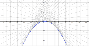
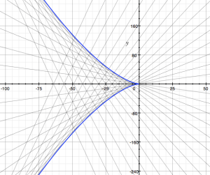
Clairaut f(t)=t^2 Clairaut equation f(t)=t^3

For the F(y’) = [y’]²functional form, you have a parabola (i.e. the graph of a quadratic function indeed) as the envelope of all of the straight lines. As for the F(y’) = [y’]³function, well… I am not sure. It reminds me of those plastic French curves we used as little kids to make all kinds of silly drawings. It also reminds me of those drawings we had to make in high school on engineering graph paper using an expensive 0.1 or 0.05 mm pen. 🙂

In any case, we’ve got quite a collection of first-order DEs now – linear, separable, exact, homogeneous, Bernouilli-type, isobaric, Clairaut-type, … – and so I think I should really stop now. Remember I haven’t started talking about higher-order DEs (e.g. second-order DEs) as yet, and I haven’t talked about partial differential equations either, and so you can imagine that the universe of differential equations is much and much larger than what this brief overview here suggests. Expect much more to come as I’ll dig into it!

Post Scriptum 2: There is a second thing I wanted to jot down somewhere, and this post may be the appropriate place. Let me ask you something: have you never wondered why the same long S symbol (i.e. the summation or integration symbol ∫) is used to denote both definite and indefinite integrals? I did. I mean the following: when we write ∫f(x)dx or ∫_{[a, b]}f(x)dx, we refer to two very different things, don’t we? Things that, at first sight, have nothing to do with each other.

Huh?

Well… Think about it. When we write ∫f(x)dx, then we actually refer to infinitely many functions F₁(x), F₂(x), F₃(x), etcetera (we generally write them as F(x) + c, because they differ by a constant only) which all belong to the same ‘family’ because they all have the same derivative, namely that function f(x) in the integrand. So we have F₁‘(x) = F₂‘(x) = F₃‘(x) = … = F'(x) = f(x). The graphs of these functions cover the whole plane, and we can say all kinds of things about them, but it is not obvious that these functions can be related to some sum, finite or infinite. Indeed, when we look for those functions by solving, for example, an integral such as ∫(xe^6x+x⁵/3+√x)dx, we use a lot of rules and various properties of functions (this one will involve integration by parts for example) but nothing of that reminds us, not even remotely, of doing some kind of finite or infinite sum.

On the other hand, ∫_{[a, b]}f(x)dx, i.e. the definite integral of f(x) over the interval [a, b], yields a real number with a very specific meaning: it’s the area between point a and point b under the graph y = f(x), and the long S symbol (i.e. the summation symbol ∫) is particularly appropriate because the expression ∫_{[a, b]}f(x)dx stands for an infinite sum indeed. That’s why Leibniz chose the symbol back in 1675!

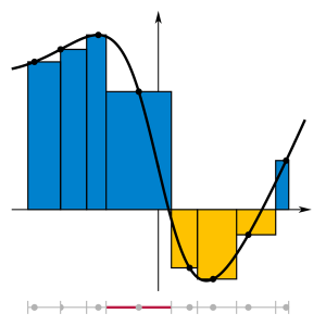
Let me give an example here. Let x be the distance which an object has traveled since we started observing it. Now, that distance is equal to an infinite sum which we can write as ∑v(t)Δt, . What we do here amounts to multiplying the speed v at time t, i.e. v(t), with (the length of) the time interval Δt over an infinite number of little time intervals, and then we sum all those products to get the total distance. If we use the differential notation (d) for infinitesimally small quantities (dv, dx, dt etcetera), then this distance x will be equal to the sum of all little distances dx = v(t)dt. So we have an infinite sum indeed which, using the long S (i.e. Leibniz’s summation symbol), we can write as ∑v(t)dt = ∑dx = ∫_{[0, t]}v(t)dt = ∫_{[0, t]}dx = x(t).

The illustration below gives an idea of how this works. The black curve is the v(t) function, so velocity (vertical axis) as a function of time (horizontal axis). Don’t worry about the function going negative: negative velocity would mean that we allow our object to reverse direction. As you can see, the value of v(t) is the (approximate) height of each of these rectangles (note that we take irregular partitions here, but that doesn’t matter), and then just imagine that the time intervals Δt (i.e. the width of the rectangular areas) become smaller and smaller – infinitesimally small in fact.

I guess I don’t need to be more explicit here. The point is that we have such infinite sum interpretation for the definite integral only, not for an indefinite one. So why would we use the same summation symbol ∫ for the indefinite integral? Why wouldn’t we use some other symbol for it (because it is something else, isn’t it?)? Or, if we wouldn’t want to introduce any new symbols (because we’ve got quite a bunch already here), then why wouldn’t we combine the common inverse function symbol (i.e. f^-1) and the differentiation operator D, D_xor d/dx, so we would write D^-1f(x) or D_x^-1instead of ∫f(x)dx? If we would do that, we would write the Fundamental Theorem of Calculus, which you obviously know (as you need it to solve definite integrals), as:

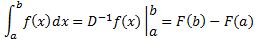
You have seen this formula, haven’t you? Except for the D^-1f(x) notation of course. This Theorem tells us that, to solve the definite integral on the left-hand side, we should just (i) take an antiderivative of f(x) (and it really doesn’t matter which one because the constant c will appear two times in the F(b) – F(a) equation, as c — c = 0 to be precise, and, hence, this constant just vanishes, regardless of its value), (ii) plug in the values a and b, (iii) subtract one from the other (i.e. F(a) from F(b), not the other way around—otherwise we’ll have the sign of the integral wrong), and there we are: we’ve got the answer—for our definite integral that is.

But so I am not using the standard ∫ symbol for the antiderivative above. I am using… well… a new symbol, D^-1, which, in my view, makes it clear what we have to do, and that is to find an antiderivative of f(x) so we can solve that definite integral. [Note that, if we’d want to keep track of what variable we’re integrating over (in case we’d be dealing with partial differential equations for instance, or if it would not be sufficiently clear from the context), we should use the D_x^-1notation, rather than just D.]

OK. You may think this is hairsplitting. What’s in a name after all? Or in a symbol in this case? Well… In math, you need to make sure that your notations make perfect sense and that you don’t write things that may be confusing.

That being said, there’s actually a very good reason to re-use the long S symbol for indefinite integrals also.

Huh? Why? You just said the definite and indefinite integral are two very different things and so that’s why you’d rather see that new D^-1f(x) notation instead of ∫f(x)dx !?

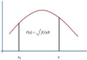
Well… Yes and no. You may or may not remember from your high school course in calculus or analysis that, in order to get to that fundamental theorem of calculus, we need the following ‘intermediate’ result: IF we define a function F(x) in some interval [a, b] as F(x) = ∫_[a, x]f(t)dt (so a ≤ x ≤ b and a ≤ t ≤ x) — so, in other words, we’ve got a definite integral here with some fixed value a as the lower boundary but with the variable x itself as the upper boundary (so we have x instead of the fixed value b, and b now only serves as the upper limit of the interval over which we’re defining this new function F(x) here) — THEN it’s easy to show that the derivative of this F(x) function will be equal to f(x), so we’ll find that F'(x) = f(x).

In other words, F(x) = ∫_[a, x]f(t)dt is, quite obviously, one of the (infinitely many) antiderivatives of f(x), and if you’d wonder which one, well… That obviously depends on the value of a that we’d be picking. So there actually is a pretty straightforward relationship between the definite and indefinite integral: we can find an antiderivative F(x) + c of a function f(x) by evaluating a definite integral from some fixed point a to the variable x itself, as illustrated below.

Now, remember that we just need one antiderivative to solve a definite integral, not the whole family, and which one we’ll get will depend on that value a (or x₀as that fixed point is being referred to in the formula used the illustration above), so it will depend on what choice we make there for the lower boundary. Indeed, you can work that out for yourself by just solving ∫_[x₀, x]f(t)dt for two different values of x₀(i.e. a and b in the example below):

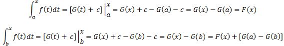
The point is that we can get all of the antiderivatives of f(x) through that definite integral: it just depends on a judicious choice of x₀ but so you’ll get the same family of functions F(x) + c. Hence, it is logical to use the same summation symbol, but with no bounds mentioned, to designate the whole family of antiderivatives. So, writing the Fundamental Theorem of Calculus as

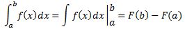
instead of that alternative with the D^-1f(x) notation does make sense. 🙂

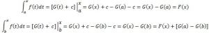
Let me wrap up this conversation by noting that the above-mentioned ‘intermediate’ result (I mean F(x) = ∫_[a, x]f(t)dt with F'(x) = f(x) here) is actually not ‘intermediate’ at all: it is equivalent to the fundamental theorem of calculus itself (indeed, the author of the Wikipedia article of the fundamental theorem of calculus presents the expression above as a ‘corollary’ to the F(x) = ∫_[a, x]f(t)dt result, which he or she presents as the theorem itself). So, if you’ve been able to prove the ‘intermediate’ result, you’ve also proved the theorem itself. One can easily see that by verifying the identities below:

Huh? Is this legal? It is. Just jot down a graph with some function f(t) and the values a, x and b, and you’ll see it all makes sense. 🙂