A Zitterbewegung model of the neutron

As part of my ventures into QCD, I quickly developed a Zitterbewegung model of the neutron, as a complement to my first sketch of a deuteron nucleus. The math of orbitals is interesting. Whatever field you have, one can model is using a coupling constant between the proportionality coefficient of the force, and the charge it acts on. That ties it nicely with my earlier thoughts on the meaning of the fine-structure constant.

My realist interpretation of quantum physics focuses on explanations involving the electromagnetic force only, but the matter-antimatter dichotomy still puzzles me very much. Also, the idea of virtual particles is no longer anathema to me, but I still want to model them as particle-field interactions and the exchange of real (angular or linear) momentum and energy, with a quantization of momentum and energy obeying the Planck-Einstein law.

The proton model will be key. We cannot explain it in the typical ‘mass without mass’ model of zittering charges: we get a 1/4 factor in the explanation of the proton radius, which is impossible to get rid of unless we assume some ‘strong’ force come into play. That is why I prioritize a ‘straight’ attack on the electron and the proton-electron bond in a primitive neutron model.

The calculation of forces inside a muon-electron and a proton (see ) is an interesting exercise: it is the only thing which explains why an electron annihilates a positron but electrons and protons can live together (the ‘anti-matter’ nature of charged particles only shows because of opposite spin directions of the fields – so it is only when the ‘structure’ of matter-antimatter pairs is different that they will not annihilate each other).

[…]

In short, 2021 will be an interesting year for me. The intent of my last two papers (on the deuteron model and the primitive neutron model) was to think of energy values: the energy value of the bond between electron and proton in the neutron, and the energy value of the bond between proton and neutron in a deuteron nucleus. But, yes, the more fundamental work remains to be done !

Cheers – Jean-Louis

An introduction to virtual particles (2)

Pre-script (dated 26 June 2020): Our ideas have evolved into a full-blown realistic (or classical) interpretation of all things quantum-mechanical. In addition, I note the dark force has amused himself by removing some material. So no use to read this. Read my recent papers instead. 🙂

Original post:

When reading quantum mechanics, it often feels like the more you know, the less you understand. My reading of the Yukawa theory of force, as an exchange of virtual particles (see my previous post), must have left you with many questions. Questions I can’t answer because… Well… I feel as much as a fool as you do when thinking about it all. Yukawa first talks about some potential – which we usually think of as being some scalar function – and then suddenly this potential becomes a wavefunction. Does that make sense? And think of the mass of that ‘virtual’ particle: the rest mass of a neutral pion is about 135 MeV. That’s an awful lot – at the (sub-)atomic scale that is: it’s equivalent to the rest mass of some 265 electrons!

But… Well… Think of it: the use of a static potential when solving Schrödinger’s equation for the electron orbitals around a hydrogen nucleus (a proton, basically) also raises lots of questions: if we think of our electron as a point-like particle being first here and then there, then that’s also not very consistent with a static (scalar) potential either!

One of the weirdest aspects of the Yukawa theory is that these emissions and absorptions of virtual particles violate the energy conservation principle. Look at the animation once again (below): it sort of assumes a rather heavy particle – consisting of a d- or u-quark and its antiparticle – is emitted – out of nothing, it seems – to then vanish as the antiparticle is destroyed when absorbed. What about the energy balance here: are we talking six quarks (the proton and the neutron), or six plus two? Nuclear_Force_anim_smaller Now that we’re talking mass, note a neutral pion (π⁰) may either be a uū or a dđ combination, and that the mass of a u-quark and a d-quark is only 2.4 and 4.8 MeV – so the binding energy of the constituent parts of this π⁰particle is enormous: it accounts for most of its mass.

The thing is… While we’ve presented the π⁰particle as a virtual particle here, you should also note we find π⁰particles in cosmic rays. Cosmic rays are particle rays, really: beams of highly energetic particles. Quite a bunch of them are just protons that are being ejected by our Sun. [The Sun also ejects electrons – as you might imagine – but let’s think about the protons here first.] When these protons hit an atom or a molecule in our atmosphere, they usually break up in various particles, including our π⁰particle, as shown below. 850px-Atmospheric_Collision

So… Well… How can we relate these things? What is going on, really, inside of that nucleus?

Well… I am not sure. Aitchison and Hey do their utmost to try to explain the pion – as a virtual particle, that is – in terms of energy fluctuations that obey the Uncertainty Principle for energy and time: ΔE·Δt ≥ ħ/2. Now, I find such explanations difficult to follow. Such explanations usually assume any measurement instrument – measuring energy, time, momentum of distance – measures those variables on some discrete scale, which implies some uncertainty indeed. But that uncertainty is more like an imprecision, in my view. Not something fundamental. Let me quote Aitchison and Hey:

“Suppose a device is set up capable of checking to see whether energy is, in fact, conserved while the pion crosses over.. The crossing time Δt must be at least r/c, where r is the distance apart of the nucleons. Hence, the device must be capable of operating on a time scale smaller than Δt to be able to detect the pion, but it need not be very much less than this. Thus the energy uncertainty in the reading by the device will be of the order ΔE ∼ ħ/Δt) = ħ·(c/r).”

As said, I find such explanations really difficult, although I can sort of sense some of the implicit assumptions. As I mentioned a couple of times already, the E = m·c² equation tells us energy is mass in motion, somehow: some weird two-dimensional oscillation in spacetime. So, yes, we can appreciate we need some time unit to count the oscillations – or, equally important, to measure their amplitude.

[…] But… Well… This falls short of a more fundamental explanation of what’s going on. I like to think of Uncertainty in terms of Planck’s constant itself: ħ or h or – as you’ll usually see it – as half of that value: ħ/2. [The Stern-Gerlach experiment implies it’s ħ/2, rather than h/2 or ħ or h itself.] The physical dimension of Planck’s constant is action: newton times distance times time. I also like to think action can express itself in two ways: as (1) some amount of energy (ΔE: some force of some distance) over some time (Δt) or, else, as (2) some momentum (Δp: some force during some time) over some distance (Δs). Now, if we equate ΔE with the energy of the pion (135 MeV), then we may calculate the order of magnitude of Δt from ΔE·Δt ≥ ħ/2 as follows:

Δt = (ħ/2)/(135 MeV) ≈ (3.291×10⁻¹⁶eV·s)/(134.977×10⁶eV) ≈ 0.02438×10⁻²²s

Now, that’s an unimaginably small time unit – but much and much larger than the Planck time (the Planck time unit is about 5.39 × 10⁻⁴⁴ s). The corresponding distance r is equal to r = Δt·c = (0.02438×10⁻²²s)·(2.998×10⁸m/s) ≈ 0.0731×10⁻¹⁴ m = 0.731 fm. So… Well… Yes. We got the answer we wanted… So… Well… We should be happy about that but…

Well… I am not. I don’t like this indeterminacy. This randomness in the approach. For starters, I am very puzzled by the fact that the lifetime of the actual π⁰particle we see in the debris of proton collisions with other particles as cosmic rays enter the atmosphere is like 8.4×10⁻¹⁷ seconds, so that’s like 35 million times longer than the Δt = 0.02438×10⁻²²s we calculated above.

Something doesn’t feel right. I just can’t see the logic here. Sorry. I’ll be back.

An introduction to virtual particles

Original post:

We are going to venture beyond quantum mechanics as it is usually understood – covering electromagnetic interactions only. Indeed, all of my posts so far – a bit less than 200, I think 🙂 – were all centered around electromagnetic interactions – with the model of the hydrogen atom as our most precious gem, so to speak.

In this post, we’ll be talking the strong force – perhaps not for the first time but surely for the first time at this level of detail. It’s an entirely different world – as I mentioned in one of my very first posts in this blog. Let me quote what I wrote there:

“The math describing the ‘reality’ of electrons and photons (i.e. quantum mechanics and quantum electrodynamics), as complicated as it is, becomes even more complicated – and, important to note, also much less accurate – when it is used to try to describe the behavior of quarks. Quantum chromodynamics (QCD) is a different world. […] Of course, that should not surprise us, because we’re talking very different order of magnitudes here: femtometers (10^–15 m), in the case of electrons, as opposed to attometers (10^–18 m) or even zeptometers (10^–21 m) when we’re talking quarks.”

In fact, the femtometer scale is used to measure the radius of both protons as well as electrons and, hence, is much smaller than the atomic scale, which is measured in nanometer (1 nm = 10⁻⁹m). The so-called Bohr radius for example, which is a measure for the size of an atom, is measured in nanometer indeed, so that’s a scale that is a million times larger than the femtometer scale. This gap in the scale effectively separates entirely different worlds. In fact, the gap is probably as large a gap as the gap between our macroscopic world and the strange reality of quantum mechanics. What happens at the femtometer scale, really?

The honest answer is: we don’t know, but we do have models to describe what happens. Moreover, for want of better models, physicists sort of believe these models are credible. To be precise, we assume there’s a force down there which we refer to as the strong force. In addition, there’s also a weak force. Now, you probably know these forces are modeled as interactions involving an exchange of virtual particles. This may be related to what Aitchison and Hey refer to as the physicist’s “distaste for action-at-a-distance.” To put it simply: if one particle – through some force – influences some other particle, then something must be going on between the two of them.

Of course, now you’ll say that something is effectively going on: there’s the electromagnetic field, right? Yes. But what’s the field? You’ll say: waves. But then you know electromagnetic waves also have a particle aspect. So we’re stuck with this weird theoretical framework: the conceptual distinction between particles and forces, or between particle and field, are not so clear. So that’s what the more advanced theories we’ll be looking at – like quantum field theory – try to bring together.

Note that we’ve been using a lot of confusing and/or ambiguous terms here: according to at least one leading physicist, for example, virtual particles should not be thought of as particles! But we’re putting the cart before the horse here. Let’s go step by step. To better understand the ‘mechanics’ of how the strong and weak interactions are being modeled in physics, most textbooks – including Aitchison and Hey, which we’ll follow here – start by explaining the original ideas as developed by the Japanese physicist Hideki Yukawa, who received a Nobel Prize for his work in 1949.

So what is it all about? As said, the ideas – or the model as such, so to speak – are more important than Yukawa’s original application, which was to model the force between a proton and a neutron. Indeed, we now explain such force as a force between quarks, and the force carrier is the gluon, which carries the so-called color charge. To be precise, the force between protons and neutrons – i.e. the so-called nuclear force – is now considered to be a rather minor residual force: it’s just what’s left of the actual strong force that binds quarks together. The Wikipedia article on this has some good text and a really nice animation on this. But… Well… Again, note that we are only interested in the model right now. So how does that look like?

First, we’ve got the equivalent of the electric charge: the nucleon is supposed to have some ‘strong’ charge, which we’ll write as g_s. Now you know the formulas for the potential energy – because of the gravitational force – between two masses, or the potential energy between two charges – because of the electrostatic force. Let me jot them down once again:

U(r) = –G·M·m/r
U(r) = (1/4πε₀)·q₁·q₂/r

The two formulas are exactly the same. They both assume U = 0 for r → ∞. Therefore, U(r) is always negative. [Just think of q₁ and q₂ as opposite charges, so the minus sign is not explicit – but it is also there!] We know that U(r) curve will look like the one below: some work (force times distance) is needed to move the two charges some distance away from each other – from point 1 to point 2, for example. [The distance r is x here – but you got that, right?]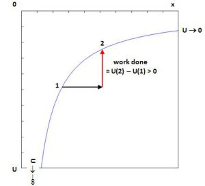 potential energy

Now, physics textbooks – or other articles you might find, like on Wikipedia – will sometimes mention that the strong force is non-linear, but that’s very confusing because… Well… The electromagnetic force – or the gravitational force – aren’t linear either: their strength is inversely proportional to the square of the distance and – as you can see from the formulas for the potential energy – that 1/r factor isn’t linear either. So that isn’t very helpful. In order to further the discussion, I should now write down Yukawa’s hypothetical formula for the potential energy between a neutron and a proton, which we’ll refer to, logically, as the n-p potential: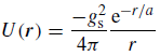The −g_s² factor is, obviously, the equivalent of the q₁·q₂ product: think of the proton and the neutron having equal but opposite ‘strong’ charges. The 1/4π factor reminds us of the Coulomb constant: k_e= 1/4πε₀. Note this constant ensures the physical dimensions of both sides of the equation make sense: the dimension of ε₀ is N·m²/C², so U(r) is – as we’d expect – expressed in newton·meter, or joule. We’ll leave the question of the units for g_s open – for the time being, that is. [As for the 1/4π factor, I am not sure why Yukawa put it there. My best guess is that he wanted to remind us some constant should be there to ensure the units come out alright.]

So, when everything is said and done, the big new thing is the e^−r/a/r factor, which replaces the usual 1/r dependency on distance. Needless to say, e is Euler’s number here – not the electric charge. The two green curves below show what the e^−r/a factor does to the classical 1/r function for a = 1 and a = 0.1 respectively: smaller values for a ensure the curve approaches zero more rapidly. In fact, for a = 1, e^−r/a/r is equal to 0.368 for r = 1, and remains significant for values r that are greater than 1 too. In contrast, for a = 0.1, e^−r/a/r is equal to 0.004579 (more or less, that is) for r = 4 and rapidly goes to zero for all values greater than that.

graph 1 graph 2 Aitchison and Hey call a, therefore, a range parameter: it effectively defines the range in which the n-p potential has a significant value: outside of the range, its value is, for all practical purposes, (close to) zero. Experimentally, this range was established as being more or less equal to r ≤ 2 fm. Needless to say, while this range factor may do its job, it’s obvious Yukawa’s formula for the n-p potential comes across as being somewhat random: what’s the theory behind? There’s none, really. It makes one think of the logistic function: the logistic function fits many statistical patterns, but it is (usually) not obvious why.

Next in Yukawa’s argument is the establishment of an equivalent, for the nuclear force, of the Poisson equation in electrostatics: using the E = –∇Φ formula, we can re-write Maxwell’s ∇•E = ρ/ε₀ equation (aka Gauss’ Law) as ∇•E = –∇•∇Φ = –∇²Φ ⇔ ∇²Φ= –ρ/ε₀ indeed. The divergence operator the ∇• operator gives us the volume density of the flux of E out of an infinitesimal volume around a given point. [You may want to check one of my post on this. The formula becomes somewhat more obvious if we re-write it as ∇•E·dV = –(ρ·dV)/ε₀: ∇•E·dV is then, quite simply, the flux of E out of the infinitesimally small volume dV, and the right-hand side of the equation says this is given by the product of the charge inside (ρ·dV) and 1/ε₀, which accounts for the permittivity of the medium (which is the vacuum in this case).] Of course, you will also remember the ∇Φ notation: ∇ is just the gradient (or vector derivative) of the (scalar) potential Φ, i.e. the electric (or electrostatic) potential in a space around that infinitesimally small volume with charge density ρ. So… Well… The Poisson equation is probably not so obvious as it seems at first (again, check my post on it on it for more detail) and, yes, that ∇• operator – the divergence operator – is a pretty impressive mathematical beast. However, I must assume you master this topic and move on. So… Well… I must now give you the equivalent of Poisson’s equation for the nuclear force. It’s written like this: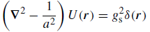What the heck? Relax. To derive this equation, we’d need to take a pretty complicated détour, which we won’t do. [See Appendix G of Aitchison and Grey if you’d want the details.] Let me just point out the basics:

1. The Laplace operator (∇²) is replaced by one that’s nearly the same: ∇² − 1/a². And it operates on the same concept: a potential, which is a (scalar) function of the position r. Hence, U(r) is just the equivalent of Φ.

2. The right-hand side of the equation involves Dirac’s delta function. Now that’s a weird mathematical beast. Its definition seems to defy what I refer to as the ‘continuum assumption’ in math. I wrote a few things about it in one of my posts on Schrödinger’s equation – and I could give you its formula – but that won’t help you very much. It’s just a weird thing. As Aitchison and Grey write, you should just think of the whole expression as a finite range analogue of Poisson’s equation in electrostatics. So it’s only for extremely small r that the whole equation makes sense. Outside of the range defined by our range parameter a, the whole equation just reduces to 0 = 0 – for all practical purposes, at least.

Now, of course, you know that the neutron and the proton are not supposed to just sit there. They’re also in these sort of intricate dance which – for the electron case – is described by some wavefunction, which we derive as a solution from Schrödinger’s equation. So U(r) is going to vary not only in space but also in time and we should, therefore, write it as U(r, t). Now, we will, of course, assume it’s going to vary in space and time as some wave and we may, therefore, suggest some wave equation for it. To appreciate this point, you should review some of the posts I did on waves. More in particular, you may want to review the post I did on traveling fields, in which I showed you the following: if we see an equation like:then the function ψ(x, t) must have the following general functional form:Any function ψ like that will work – so it will be a solution to the differential equation – and we’ll refer to it as a wavefunction. Now, the equation (and the function) is for a wave traveling in one dimension only (x) but the same post shows we can easily generalize to waves traveling in three dimensions. In addition, we may generalize the analyse to include complex-valued functions as well. Now, you will still be shocked by Yukawa’s field equation for U(r, t) but, hopefully, somewhat less so after the above reminder on how wave equations generally look like: 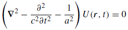Yukawa wave equation As said, you can look up the nitty-gritty in Aitchison and Grey (or in its appendices) but, up to this point, you should be able to sort of appreciate what’s going on without getting lost in it all. Yukawa’s next step – and all that follows – is much more baffling. We’d think U, the nuclear potential, is just some scalar-valued wave, right? It varies in space and in time, but… Well… That’s what classical waves, like water or sound waves, for example do too. So far, so good. However, Yukawa’s next step is to associate a de Broglie-type wavefunction with it. Hence, Yukawa imposes solutions of the type:What? Yes. It’s a big thing to swallow, and it doesn’t help most physicists refer to U as a force field. A force and the potential that results from it are two different things. To put it simply: the force on an object is not the same as the work you need to move it from here to there. Force and potential are related but different concepts. Having said that, it sort of make sense now, doesn’t it? If potential is energy, and if it behaves like some wave, then we must be able to associate it with a de Broglie-type particle. This U-quantum, as it is referred to, comes in two varieties, which are associated with the ongoing absorption-emission process that is supposed to take place inside of the nucleus (depicted below):

p + U⁻ → n and n + U⁺ → p

absorption emission

It’s easy to see that the U⁻ and U⁺ particles are just each other’s anti-particle. When thinking about this, I can’t help remembering Feynman, when he enigmatically wrote – somewhere in his Strange Theory of Light and Matter – that an anti-particle might just be the same particle traveling back in time. In fact, the exchange here is supposed to happen within a time window that is so short it allows for the brief violation of the energy conservation principle.

Let’s be more precise and try to find the properties of that mysterious U-quantum. You’ll need to refresh what you know about operators to understand how substituting Yukawa’s de Broglie wavefunction in the complicated-looking differential equation (the wave equation) gives us the following relation between the energy and the momentum of our new particle: mass 1 Now, it doesn’t take too many gimmicks to compare this against the relativistically correct energy-momentum relation:Combining both gives us the associated (rest) mass of the U-quantum: rest mass For a ≈ 2 fm, m_U is about 100 MeV. Of course, it’s always to check the dimensions and calculate stuff yourself. Note the physical dimension of ħ/(a·c) is N·s²/m = kg (just think of the F = m·a formula). Also note that N·s²/m = kg = (N·m)·s²/m²= J/(m²/s²), so that’s the [E]/[c²] dimension. The calculation – and interpretation – is somewhat tricky though: if you do it, you’ll find that:

ħ/(a·c) ≈ (1.0545718×10⁻³⁴ N·m·s)/[(2×10⁻¹⁵ m)·(2.997924583×10⁸ m/s)] ≈ 0.176×10⁻²⁷kg

Now, most physics handbooks continue that terrible habit of writing particle weights in eV, rather than using the correct eV/c² unit. So when they write: m_U is about 100 MeV, they actually mean to say that it’s 100 MeV/c². In addition, the eV is not an SI unit. Hence, to get that number, we should first write 0.176×10⁻²⁷kg as some value expressed in J/c², and then convert the joule (J) into electronvolt (eV). Let’s do that. First, note that c² ≈ 9×10¹⁶ m²/s², so 0.176×10⁻²⁷kg ≈ 1.584×10⁻¹¹J/c². Now we do the conversion from joule to electronvolt. We get: (1.584×10⁻¹¹J/c²)·(6.24215×10¹⁸ eV/J) ≈ 9.9×10⁷ eV/c² = 99 MeV/c². Bingo! So that was Yukawa’s prediction for the nuclear force quantum.

Of course, Yukawa was wrong but, as mentioned above, his ideas are now generally accepted. First note the mass of the U-quantum is quite considerable: 100 MeV/c² is a bit more than 10% of the individual proton or neutron mass (about 938-939 MeV/c²). While the binding energy causes the mass of an atom to be less than the mass of their constituent parts (protons, neutrons and electrons), it’s quite remarkably that the deuterium atom – a hydrogen atom with an extra neutron – has an excess mass of about 13.1 MeV/c², and a binding energy with an equivalent mass of only 2.2 MeV/c². So… Well… There’s something there.

As said, this post only wanted to introduce some basic ideas. The current model of nuclear physics is represented by the animation below, which I took from the Wikipedia article on it. The U-quantum appears as the pion here – and it does not really turn the proton into a neutron and vice versa. Those particles are assumed to be stable. In contrast, it is the quarks that change color by exchanging gluons between each other. And we know look at the exchange particle – which we refer to as the pion – between the proton and the neutron as consisting of two quarks in its own right: a quark and a anti-quark. So… Yes… All weird. QCD is just a different world. We’ll explore it more in the coming days and/or weeks. 🙂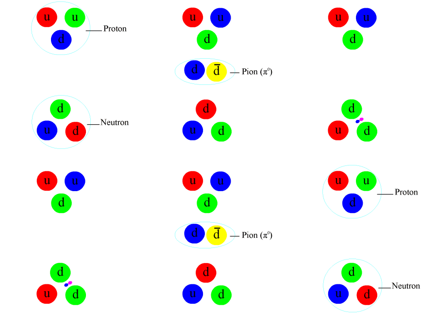 Nuclear_Force_anim_smaller An alternative – and simpler – way of representing this exchange of a virtual particle (a neutral pion in this case) is obtained by drawing a so-called Feynman diagram: Pn_scatter_pi0 OK. That’s it for today. More tomorrow. 🙂

Some content on this page was disabled on June 20, 2020 as a result of a DMCA takedown notice from Michael A. Gottlieb, Rudolf Pfeiffer, and The California Institute of Technology. You can learn more about the DMCA here:

https://wordpress.com/support/copyright-and-the-dmca/
Some content on this page was disabled on June 20, 2020 as a result of a DMCA takedown notice from Michael A. Gottlieb, Rudolf Pfeiffer, and The California Institute of Technology. You can learn more about the DMCA here:

https://wordpress.com/support/copyright-and-the-dmca/

An introduction to virtual particles

In one of my posts on the rules of quantum math, I introduced the propagator function, which gives us the amplitude for a particle to go from one place to another. It looks like this:

The r₁and r₂ vectors are, obviously, position vectors describing (1) where the particle is right now, so the initial state is written as |r₁〉, and (2) where it might go, so the final state is |r₂〉. Now we can combine this with the analysis in my previous post to think about what might happen when an electron sort of ‘jumps’ from one state to another. It’s a rather funny analysis, but it will give you some feel of what these so-called ‘virtual’ particles might represent.

Let’s first look at the shape of that function. The e^{(i/ħ)·(p∙r₁₂)}function in the numerator is now familiar to you. Note the r₁₂in the argument, i.e. the vector pointing from r₁ to r₂. The p∙r₁₂ dot product equals |p|∙|r₁₂|·cosθ = p∙r₁₂·cosθ, with θ the angle between p and r₁₂. If the angle is the same, then cosθ is equal to 1. If the angle is π/2, then it’s 0, and the function reduces to 1/r₁₂. So the angle θ, through the cosθ factor, sort of scales the spatial frequency. Let me try to give you some idea of how this looks like by assuming the angle between p and r₁₂ is the same, so we’re looking at the space in the direction of the momentum only and |p|∙|r₁₂|·cosθ = p∙r₁₂. Now, we can look at the p/ħ factor as a scaling factor, and measure the distance x in units defined by that scale, so we write: x = p∙r₁₂/ħ. The whole function, including the denominator, then reduces to (ħ/p)·e^i∙x/x = (ħ/p)·cos(x)/x + i·(ħ/p)·sin(x)/x, and we just need to square this to get the probability. All of the graphs are drawn hereunder: I’ll let you analyze them. [Note that the graphs do not include the ħ/p factor, which you may look at as yet another scaling factor.] You’ll see – I hope! – that it all makes perfect sense: the probability quickly drops off with distance, both in the positive as well as in the negative x-direction, while going to infinity when very near, i.e. for very small x. [Note that the absolute square, using cos(x)/x and sin(x)/xyields the same graph as squaring 1/x—obviously!]

Now, this propagator function is not dependent on time: it’s only the momentum that enters the argument. Of course, we assume p to be some positive real number. Of course?

This is where Feynman starts an interesting conversation. In the previous post, we studied a model in which we had two protons, and one electron jumping from one to another, as shown below.

This model told us the equilibrium state is a stable ionized hydrogen molecule (so that’s an H₂⁺molecule), with an interproton distance that’s equal to 1 Ångstrom – so that’s like twice the size of a hydrogen atom (which we simply write as H) – and an energy that’s 2.72 eV less than the energy of a hydrogen atom and a proton (so that’s not an H₂⁺molecule but a system consisting of a separate hydrogen atom and a proton). The why and how of that equilibrium state is illustrated below. [For more details, see my previous post.]

Now, the model implies there is a sort of attractive force pulling the two protons together even when the protons are at larger distances than 1 Å. One can see that from the graph indeed. Now, we would not associate any molecular orbital with those distances, as the system is, quite simply, not a molecule but a separate hydrogen atom and a proton. Nevertheless, the amplitude A is non-zero, and so we have an electron jumping back and forth.

We know how that works from our post on tunneling: particles can cross an energy barrier and tunnel through. One of the weird things we had to consider when a particle crosses such potential barrier, is that the momentum factor p in its wavefunction was some pure imaginary number, which we wrote as p = i·p’. We then re-wrote that wavefunction as a·e⁻ⁱ^θ = a·e⁻ⁱ^[^{(E/ħ)∙t − (i·p’/ħ)x]} = a·e⁻ⁱ^(E/ħ)∙t·e^{i²·p’·x/ħ} = a·e⁻ⁱ^(E/ħ)∙t·e^{−p’·x/ħ}. The e^{−p’·x/ħ} factor in this formula is a real-valued exponential function, that sort of ‘kills’ our wavefunction as we move across the potential barrier, which is what is illustrated below: if the distance is too large, then the amplitude for tunneling goes to zero.

From a mathematical point of view, the analysis of our electron jumping back and forth is very similar. However, there are differences too. We can’t really analyze this in terms of a potential barrier in space. The barrier is the potential energy of the electron itself: it’s happy when it’s bound, because its energy then contributes to a reduction of the total energy of the hydrogen atomic system that is equal to the ionization energy, or the Rydberg energy as it’s called, which is equal to not less than 13.6 eV (which, as mentioned, is pretty big at the atomic level). Well… We can take that propagator function (1/r)·e^{(i/ħ)·p∙r} (note the argument has no minus sign: it can be quite tricky!), and just fill in the value for the momentum of the electron.

Huh? What momentum? It’s got no momentum to spare. On the contrary, it wants to stay with the proton, so it has no energy whatsoever to escape. Well… Not in quantum mechanics. In quantum mechanics it can use all its potential energy and convert it into kinetic energy, so it can get away from its proton and convert the energy that’s being released into kinetic energy.

But there is no release of energy! The energy is negative!

Exactly! You’re right. So we boldly write: K.E. = m·v²/2 = p²/(2m) = −13.6 eV, and, because we’re working with complex numbers, we can take a square root of negative number, using the definition of the imaginary unit: i = √(−1), so we get a purely imaginary value for the momentum p, which we write as:

p = ±i·√(2m·E_H)

The sign of p is chosen so it makes sense: our electron should go in one direction only. It’s going to be the plus sign. [If you’d take the negative root, you’d get a nonsensical propagator function.] To make a long story short, our propagator function becomes:

(1/r)·e^{(i/ħ)·i·√(2m·E_H)∙r} = (1/r)·e^{(i/ħ)·i·√(2m·E_H)∙r} = (1/r)·e^{i²/ħ·√(2m·E_H)∙r} = (1/r)·e^{−√(2m·E_H)/ħ∙r}

Of course, from a mathematical point of view, that’s the same function as e^{−p’·x/ħ}: it’s a real-valued exponential function that quickly dies. But it’s an amplitude alright, and it’s just like an amplitude for tunneling indeed: if the distance is too large, then the amplitude goes to zero. The final cherry on the cake, of course, is to write:

A ∼ (1/r)·e^{−√(2m·E_H)/ħ∙r}

Well… No. It gets better. This amplitude is an amplitude for an electron bond between the two protons which, as we know, lowers the energy of the system. By how much? Well… By A itself. Now we know that work or energy is an integral or antiderivative of force over distance, so force is the derivative of energy with respect to the distance. So we can just take the derivative of the expression above to get the force. I’ll leave that you as an exercise: don’t forget to use the product rule! 🙂

So are we done? No. First, we didn’t talk about virtual particles yet! Let me do that now. However, first note that we should add one more effect in our two-proton-one-electron system: the coulomb field (ε) caused by the bare proton will cause the hydrogen molecule to take on an induced electric dipole moment (μ), so we should integrate that in our energy equation. Feynman shows how, but I won’t bother you with that here. Let’s talk about those virtual particles. What are they?

Well… There’s various definitions, but Feynman’s definition is this one:

“There is an exchange of a virtual electron when–as here–the electron has to jump across a space where it would have a negative energy. More specifically, a ‘virtual exchange’ means that the phenomenon involves a quantum-mechanical interference between an exchanged state and a non-exchanged state.”

You’ll say: what’s virtual about it? The electron does go from one place to another, doesn’t it? Well… Yes and no. We can’t observe it while it’s supposed to be doing that. Our analysis just tells us it seems to be useful to distinguish two different states and analyze all in terms of those differential equations. Who knows what’s really going on? What’s actual and what’s virtual? We just have some ‘model’ here: a model for the interaction between a hydrogen atom and a proton. It explains the attraction between them in terms of a sort of continuous exchange of an electron, but is it real?

The point is: in physics, it’s assumed that the coulomb interaction, i.e. all of electrostatics really, comes from the exchange of virtual photons: one electron, or proton, emits a photon, and then another absorbs it in the reverse of the same reaction. Furthermore, it is assumed that the amplitude for doing so is like that formula we found for the amplitude to exchange a virtual electron, except that the rest mass of a photon is zero, and so the formula reduces to 1/r. Such simple relationship makes sense, of course, because that’s how the electrostatic potential varies in space!

That, in essence, is all what there is to the quantum-mechanical theory of electromagnetism, which Feynman refers to as the ‘particle point of view’.

So… Yes. It’s that simple. Yes! For a change! 🙂

Post scriptum: Feynman’s Lecture on virtual particles is actually focused on a model for the nuclear forces. Most of it is devoted to a discussion of the virtual ‘pion’, or π-meson, which was then, when Feynman wrote his Lectures, supposed to mediate the force between two nucleons. However, this theory is clearly outdated: nuclear forces are described by quantum chromodynamics. So I’ll just skip the Yukawa theory here. It’s actually kinda strange his theory, which he proposed in 1935, was the theory for nuclear forces for such a long time. Hence, it’s surely all very interesting from a historical point of view.