
Pre-script (dated 26 June 2020): Our ideas have evolved into a full-blown realistic (or classical) interpretation of all things quantum-mechanical. In addition, I note the dark force has amused himself by removing some material. So no use to read this. Read my recent papers instead. 🙂
Original post:
We’ve climbed a big mountain over the past few weeks, post by post, 🙂 slowly gaining height, and carefully checking out the various routes to the top. But we are there now: we finally fully understand how Maxwell’s equations actually work. Let me jot them down once more:

As for how real or unreal the E and B fields are, I gave you Feynman’s answer to it, so… Well… I can’t add to that. I should just note, or remind you, that we have a fully equivalent description of it all in terms of the electric and magnetic (vector) potential Φ and A, and so we can ask the same question about Φ and A. They explain real stuff, so they’re real in that sense. That’s what Feynman’s answer amounts to, and I am happy with it. 🙂
What I want to do here is show how we can get from those equations to some kind of wave equation: an equation that describes how a field actually travels through space. So… Well… Let’s first look at that very particular wave function we used in the previous post to prove that electromagnetic waves propagate with speed c, i.e. the speed of light. The fields were very simple: the electric field had a y-component only, and the magnetic field a z-component only. Their magnitudes, i.e. their magnitude where the field had reached, as it fills the space traveling outwards, were given in terms of J, i.e. the surface current density going in the positive y-direction, and the geometry of the situation is illustrated below.
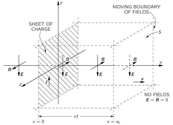
The fields were, obviously, zero where the fields had not reached as they were traveling outwards. And, yes, I know that sounds stupid. But… Well… It’s just to make clear what we’re looking at here. 🙂
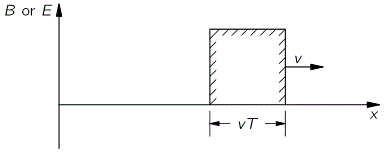
We also showed how the wave would look like if we would turn off its First Cause after some time T, so if the moving sheet of charge would no longer move after time T. We’d have the following pulse traveling through space, a rectangular shape really:
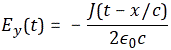
 We can imagine more complicated shapes for the pulse, like the shape shown below. J goes from one unit to two units at time t = t1 and then to zero at t = t2. Now, the illustration on the right shows the electric field as a function of x at the time t shown by the arrow. We’ve seen this before when discussing waves: if the speed of travel of the wave is equal to c, then x is equal to x = c·t, and the pattern is as shown below indeed: it mirrors what happened at the source x/c seconds ago. So we write:
This idea of using the retarded time t’ = t − x/c in the argument of a wave function f – or, what amounts to the same, using x − c/t – is key to understanding wave functions. I’ve explained this in very simple language in a post for my kids and, if you don’t get this, I recommend you check it out. What we’re doing, basically, is converting something expressed in time units into something expressed in distance units, or vice versa, using the velocity of the wave as the scale factor, so time and distance are both expressed in the same unit, which may be seconds, or meter.
To see how it works, suppose we add some time Δt to the argument of our wave function f, so we’re looking at f[x−c(t+Δt)] now, instead of f(x−ct). Now, f[x−c(t+Δt)] = f(x−ct−cΔt), so we’ll get a different value for our function—obviously! But it’s easy to see that we can restore our wave function F to its former value by also adding some distance Δx = cΔt to the argument. Indeed, if we do so, we get f[x+Δx−c(t+Δt)] = f(x+cΔt–ct−cΔt) = f(x–ct). You’ll say: t − x/c is not the same as x–ct. It is and it isn’t: any function of x–ct is also a function of t − x/c, because we can write:
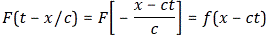
Here, I need to add something about the direction of travel. The pulse above travel in the positive x-direction, so that’s why we have x minus ct in the argument. For a wave traveling in the negative x-direction, we’ll have a wave function y = F(x+ct). In any case, I can’t dwell on this, so let me move on.
Now, Maxwell’s equations in free or empty space, where are there no charges nor currents to interact with, reduce to:
Now, how can we relate this set of complicated equations to a simple wave function? Let’s do the exercise for our simple Ey and Bz wave. Let’s start by writing out the first equation, i.e. ∇·E = 0, so we get:
![]()
Now, our wave does not vary in the y and z direction, so none of the components, including Ey and Ez depend on y or z. It only varies in the x-direction, so ∂Ey/∂y and ∂Ez/∂z are zero. Note that the cross-derivatives ∂Ey/∂z and ∂Ez/∂y are also zero: we’re talking a plane wave here, the field varies only with x. However, because ∇·E = 0, ∂Ex/∂x must be zero and, hence, Ex must be zero.
Huh? What? How is that possible? You just said that our field does vary in the x-direction! And now you’re saying it doesn’t it? Read carefully. I know it’s complicated business, but it all makes sense. Look at the function: we’re talking Ey, not Ex. Ey does vary as a function of x, but our field does not have an x-component, so Ex = 0. We have no cross-derivative ∂Ey/∂x in the divergence of E (i.e. in ∇·E = 0).
Huh? What? Let me put it differently. E has three components: Ex, Ey and Ez, and we have three space coordinates: x, y and z, so we have nine cross-derivatives. What I am saying is that all derivatives with respect to y and z are zero. That still leaves us with three derivatives: ∂Ex/∂x, ∂Ey/∂x, and ∂Ey/∂x. So… Because all derivatives in respect to y and z are zero, and because of the ∇·E = 0 equation, we know that ∂Ex/∂x must be zero. So, to make a long story short, I did not say anything about ∂Ey/∂x or ∂Ez/∂x. These may still be whatever they want to be, and they may vary in more or in less complicated ways. I’ll give an example of that in a moment.
Having said that, I do agree that I was a bit quick in writing that, because ∂Ex/∂x = 0, Ex must be zero too. Looking at the math only, Ex is not necessarily zero: it might be some non-zero constant. So… Yes. That’s a mathematical possibility. The static field from some charged condenser plate would be an example of a constant Ex field. However, the point is that we’re not looking at such static fields here: we’re talking dynamics here, and we’re looking at a particular type of wave: we’re talking a so-called plane wave. Now, the wave front of a plane wave is… Well… A plane. 🙂 So Ex is zero indeed. It’s a general result for plane waves: the electric field of a plane wave will always be at right angles to the direction of propagation.
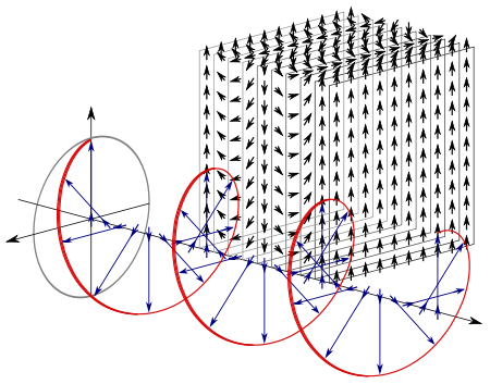
Hmm… I can feel your skepticism here. You’ll say I am arbitrarily restricting the field of analysis… Well… Yes. For the moment. It’s not a reasonable restriction though. As I mentioned above, the field of a plane wave may still vary in both the y- and z-directions, as shown in the illustration below (for which the credit goes to Wikipedia), which visualizes the electric field of circularly polarized light. In any case, don’t worry too much about. Let’s get back to the analysis. Just note we’re talking plane waves here. We’ll talk about non-plane waves i.e. incoherent light waves later. 🙂
So we have plane waves and, therefore, a so-called transverse E field which we can resolve in two components: Ey and Ez. However, we wanted to study a very simply Ey field only. Why? Remember the objective of this lesson: it’s just to show how we go from Maxwell’s equations to the wave function, and so let’s keep the analysis simple as we can for now: we can make it more general later. In fact, if we do the analysis now for non-zero Ey and zero Ez, we can do a similar analysis for non-zero Ez and zero Ey, and the general solution is going to be some superposition of two such fields, so we’ll have a non-zero Ey and Ez. Capito? 🙂 So let me write out Maxwell’s second equation, and use the results we got above, so I’ll incorporate the zero values for the derivatives with respect to y and z, and also the assumption that Ez is zero. So we get:
[By the way: note that, out of the nine derivatives, the curl involves only the (six) cross-derivatives. That’s linked to the neat separation between the curl and the divergence operator. Math is great! :-)]
Now, because of the flux rule (∇×E = –∂B/∂t), we can (and should) equate the three components of ∇×E above with the three components of –∂B/∂t, so we get:
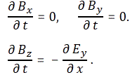
[In case you wonder what it is that I am trying to do, patience, please! We’ll get where we want to get. Just hang in there and read on.] Now, ∂Bx/∂t = 0 and ∂By/∂t = 0 do not necessarily imply that Bx and By are zero: there might be some magnets and, hence, we may have some constant static field. However, that’s a matter of choosing a reference point or, more simply, assuming that empty space is effectively empty, and so we don’t have magnets lying around and so we assume that Bx and By are effectively zero. [Again, we can always throw more stuff in when our analysis is finished, but let’s keep it simple and stupid right now, especially because the Bx = By = 0 is entirely in line with the Ex = Ez = 0 assumption.]
The equations above tell us what we know already: the E and B fields are at right angles to each other. However, note, once again, that this is a more general result for all plane electromagnetic waves, so it’s not only that very special caterpillar or butterfly field that we’re looking at it. [If you didn’t read my previous post, you won’t get the pun, but don’t worry about it. You need to understand the equations, not the silly jokes.]
OK. We’re almost there. Now we need Maxwell’s last equation. When we write it out, we get the following monstrously looking set of equations:
However, because of all of the equations involving zeroes above 🙂 only ∂Bz/∂x is not equal to zero, so the whole set reduced to only simple equation only:
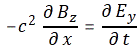
Simplifying assumptions are great, aren’t they? 🙂 Having said that, it’s easy to be confused. You should watch out for the denominators: a ∂x and a ∂t are two very different things. So we have two equations now involving first-order derivatives:
- ∂Bz/∂t = −∂Ey/∂x
- −c2∂Bz/∂x = −∂Ey/∂t
So what? Patience, please! 🙂 Let’s differentiate the first equation with respect to x and the second with respect to t. Why? Because… Well… You’ll see. Don’t complain. It’s simple. Just do it. We get:
- ∂[∂Bz/∂t]/∂x = −∂2Ey/∂x2
- ∂[−c2∂Bz/∂x]/∂t = −∂2Ey/∂x2
So we can equate the left-hand sides of our two equations now, and what we get is a differential equation of the second order that we’ve encountered already, when we were studying wave equations. In fact, it is the wave equation for one-dimensional waves:
In case you want to double-check, I did a few posts on this, but, if you don’t get this, well… I am sorry. You’ll need to do some homework. More in particular, you’ll need to do some homework on differential equations. The equation above is basically some constraint on the functional form of Ey. More in general, if we see an equation like:
then the function ψ(x, t) must be some function
![]()
So any function ψ like that will work. You can check it out by doing the necessary derivatives and plug them into the wave equation. [In case you wonder how you should go about this, Feynman actually does it for you in his Lecture on this topic, so you may want to check it there.]
In fact, the functions f(x − c/t) and g(x + c/t) themselves will also work as possible solutions. So we can drop one or the other, which amounts to saying that our ‘shape’ has to travel in some direction, rather than in both at the same time. 🙂 Indeed, from all of my explanations above, you know what f(x − c/t) represents: it’s a wave that travels in the positive x-direction. Now, it may be periodic, but it doesn’t have to be periodic. The f(x − c/t) function could represent any constant ‘shape’ that’s traveling in the positive x-direction at speed c. Likewise, the g(x + c/t) function could represent any constant ‘shape’ that’s traveling in the negative x-direction at speed c. As for super-imposing both…
Well… I suggest you check that post I wrote for my son, Vincent. It’s on the math of waves, but it doesn’t have derivatives and/or differential equations. It just explains how superimposition and all that works. It’s not very abstract, as it revolves around a vibrating guitar string. So, if you have trouble with all of the above, you may want to read that first. 🙂 The bottom line is that we can get any wavefunction we want by superimposing simple sinusoidals that are traveling in one or the other direction, and so that’s what’s the more general solution really says. Full stop. So that’s what’s we’re doing really: we add very simple waves to get very more complicated waveforms. 🙂
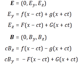
Now, I could leave it at this, but then it’s very easy to just go one step further, and that is to assume that Ez and, therefore, By are not zero. It’s just a matter of super-imposing solutions. Let me just give you the general solution. Just look at it for a while. If you understood all that I’ve said above, 20 seconds or so should be sufficient to say: “Yes, that makes sense. That’s the solution in two dimensions.” At least, I hope so! 🙂
OK. I should really stop now. But… Well… Now that we’ve got a general solution for all plane waves, why not be even bolder and think about what we could possibly say about three-dimensional waves? So then Ex and, therefore, Bx would not necessarily be zero either. After all, light can behave that way. In fact, light is likely to be non-polarized and, hence, Ex and, therefore, Bx are most probably not equal to zero!
Now, you may think the analysis is going to be terribly complicated. And you’re right. It would be if we’d stick to our analysis in terms of x, y and z coordinates. However, it turns out that the analysis in terms of vector equations is actually quite straightforward. I’ll just copy the Master here, so you can see His Greatness. 🙂
But what solution does an equation like (20.27) have? We can appreciate it’s actually three equations, i.e. one for each component, and so… Well… Hmm… What can we say about that? I’ll quote the Master on this too:
“How shall we find the general wave solution? The answer is that all the solutions of the three-dimensional wave equation can be represented as a superposition of the one-dimensional solutions we have already found. We obtained the equation for waves which move in the x-direction by supposing that the field did not depend on y and z. Obviously, there are other solutions in which the fields do not depend on x and z, representing waves going in the y-direction. Then there are solutions which do not depend on x and y, representing waves travelling in the z-direction. Or in general, since we have written our equations in vector form, the three-dimensional wave equation can have solutions which are plane waves moving in any direction at all. Again, since the equations are linear, we may have simultaneously as many plane waves as we wish, travelling in as many different directions. Thus the most general solution of the three-dimensional wave equation is a superposition of all sorts of plane waves moving in all sorts of directions.”
It’s the same thing once more: we add very simple waves to get very more complicated waveforms. 🙂
You must have fallen asleep by now or, else, be watching something else. Feynman must have felt the same. After explaining all of the nitty-gritty above, Feynman wakes up his students. He does so by appealing to their imagination:
“Try to imagine what the electric and magnetic fields look like at present in the space in this lecture room. First of all, there is a steady magnetic field; it comes from the currents in the interior of the earth—that is, the earth’s steady magnetic field. Then there are some irregular, nearly static electric fields produced perhaps by electric charges generated by friction as various people move about in their chairs and rub their coat sleeves against the chair arms. Then there are other magnetic fields produced by oscillating currents in the electrical wiring—fields which vary at a frequency of 6060 cycles per second, in synchronism with the generator at Boulder Dam. But more interesting are the electric and magnetic fields varying at much higher frequencies. For instance, as light travels from window to floor and wall to wall, there are little wiggles of the electric and magnetic fields moving along at 186,000 miles per second. Then there are also infrared waves travelling from the warm foreheads to the cold blackboard. And we have forgotten the ultraviolet light, the x-rays, and the radiowaves travelling through the room.
Flying across the room are electromagnetic waves which carry music of a jazz band. There are waves modulated by a series of impulses representing pictures of events going on in other parts of the world, or of imaginary aspirins dissolving in imaginary stomachs. To demonstrate the reality of these waves it is only necessary to turn on electronic equipment that converts these waves into pictures and sounds.
If we go into further detail to analyze even the smallest wiggles, there are tiny electromagnetic waves that have come into the room from enormous distances. There are now tiny oscillations of the electric field, whose crests are separated by a distance of one foot, that have come from millions of miles away, transmitted to the earth from the Mariner II space craft which has just passed Venus. Its signals carry summaries of information it has picked up about the planets (information obtained from electromagnetic waves that travelled from the planet to the space craft).
There are very tiny wiggles of the electric and magnetic fields that are waves which originated billions of light years away—from galaxies in the remotest corners of the universe. That this is true has been found by “filling the room with wires”—by building antennas as large as this room. Such radiowaves have been detected from places in space beyond the range of the greatest optical telescopes. Even they, the optical telescopes, are simply gatherers of electromagnetic waves. What we call the stars are only inferences, inferences drawn from the only physical reality we have yet gotten from them—from a careful study of the unendingly complex undulations of the electric and magnetic fields reaching us on earth.
There is, of course, more: the fields produced by lightning miles away, the fields of the charged cosmic ray particles as they zip through the room, and more, and more. What a complicated thing is the electric field in the space around you! Yet it always satisfies the three-dimensional wave equation.”
So… Well… That’s it for today, folks. 🙂 We have some more gymnastics to do, still… But we’re really there. Or here, I should say: on top of the peak. What a view we have here! Isn’t it beautiful? It took us quite some effort to get on top of this thing, and we’re still trying to catch our breath as we struggle with what we’ve learned so far, but it’s really worthwhile, isn’t it? 🙂
Some content on this page was disabled on June 16, 2020 as a result of a DMCA takedown notice from The California Institute of Technology. You can learn more about the DMCA here:
https://wordpress.com/support/copyright-and-the-dmca/
Some content on this page was disabled on June 16, 2020 as a result of a DMCA takedown notice from The California Institute of Technology. You can learn more about the DMCA here:https://wordpress.com/support/copyright-and-the-dmca/
Some content on this page was disabled on June 16, 2020 as a result of a DMCA takedown notice from The California Institute of Technology. You can learn more about the DMCA here:https://wordpress.com/support/copyright-and-the-dmca/
Some content on this page was disabled on June 16, 2020 as a result of a DMCA takedown notice from The California Institute of Technology. You can learn more about the DMCA here:https://wordpress.com/support/copyright-and-the-dmca/
Some content on this page was disabled on June 16, 2020 as a result of a DMCA takedown notice from The California Institute of Technology. You can learn more about the DMCA here:https://wordpress.com/support/copyright-and-the-dmca/
Some content on this page was disabled on June 16, 2020 as a result of a DMCA takedown notice from The California Institute of Technology. You can learn more about the DMCA here:https://wordpress.com/support/copyright-and-the-dmca/
Some content on this page was disabled on June 16, 2020 as a result of a DMCA takedown notice from The California Institute of Technology. You can learn more about the DMCA here:https://wordpress.com/support/copyright-and-the-dmca/
Some content on this page was disabled on June 16, 2020 as a result of a DMCA takedown notice from The California Institute of Technology. You can learn more about the DMCA here:https://wordpress.com/support/copyright-and-the-dmca/
Some content on this page was disabled on June 16, 2020 as a result of a DMCA takedown notice from The California Institute of Technology. You can learn more about the DMCA here:https://wordpress.com/support/copyright-and-the-dmca/
Some content on this page was disabled on June 20, 2020 as a result of a DMCA takedown notice from Michael A. Gottlieb, Rudolf Pfeiffer, and The California Institute of Technology. You can learn more about the DMCA here:https://wordpress.com/support/copyright-and-the-dmca/
Some content on this page was disabled on June 20, 2020 as a result of a DMCA takedown notice from Michael A. Gottlieb, Rudolf Pfeiffer, and The California Institute of Technology. You can learn more about the DMCA here:

3 thoughts on “Traveling fields: the wave equation and its solutions”