The blackbody radiation problem revisited: quantum statistics

Pre-script (dated 26 June 2020): This post got mutilated by the removal of some illustrations by the dark force. You should be able to follow the main story-line, however. If anything, the lack of illustrations might actually help you to think things through for yourself.

Original post:

The equipartition theorem – which states that the energy levels of the modes of any (linear) system, in classical as well as in quantum physics, are always equally spaced – is deep and fundamental in physics. In my previous post, I presented this theorem in a very general and non-technical way: I did not use any exponentials, complex numbers or integrals. Just simple arithmetic. Let’s go a little bit beyond now, and use it to analyze that blackbody radiation problem which bothered 19th century physicists, and which led Planck to ‘discover’ quantum physics. [Note that, once again, I won’t use any complex numbers or integrals in this post, so my kids should actually be able to read through it.]

Before we start, let’s quickly introduce the model again. What are we talking about? What’s the black box? The idea is that we add heat to atoms (or molecules) in a gas. The heat results in the atoms acquiring kinetic energy, and the kinetic theory of gases tells us that the mean value of the kinetic energy for each independent direction of motion will be equal to kT/2. The blackbody radiation model analyzes the atoms (or molecules) in a gas as atomic oscillators. Oscillators have both kinetic as well as potential energy and, on average, the kinetic and potential energy is the same. Hence, the energy in the oscillation is twice the kinetic energy, so its average energy is 〈E〉 = 2·kT/2 = kT. However, oscillating atoms implies oscillating electric charges. Now, electric charges going up and down radiate light and, hence, as light is emitted, energy flows away.

How exactly? It doesn’t matter. It is worth noting that 19th century physicists had no idea about the inner structure of an atom. In fact, at that time, the term electron had not yet been invented: the first atomic model involving electrons was the so-called plum pudding model, which J.J. Thompson advanced in 1904, and he called electrons “negative corpuscles“. And the Rutherford-Bohr model, which is the first model one can actually use to explain how and why excited atoms radiate light, came in 1913 only, so that’s long after Planck’s solution for the blackbody radiation problem, which he presented to the scientific community in December 1900. It’s really true: it doesn’t matter. We don’t need to know about the specifics. The general idea is all that matters. As Feynman puts it: it’s how “A hot stove cools on a cold night, by radiating the light into the sky, because the atoms are jiggling their charge and they continually radiate, and slowly, because of this radiation, the jiggling motion slows down.” 🙂

His subsequent description of the black box is equally simple: “If we enclose the whole thing in a box so that the light does not go away to infinity, then we can eventually get thermal equilibrium. We may either put the gas in a box where we can say that there are other radiators in the box walls sending light back or, to take a nicer example, we may suppose the box has mirror walls. It is easier to think about that case. Thus we assume that all the radiation that goes out from the oscillator keeps running around in the box. Then, of course, it is true that the oscillator starts to radiate, but pretty soon it can maintain its kT of energy in spite of the fact that it is radiating, because it is being illuminated, we may say, by its own light reflected from the walls of the box. That is, after a while there is a great deal of light rushing around in the box, and although the oscillator is radiating some, the light comes back and returns some of the energy that was radiated.”

So… That’s the model. Don’t you just love the simplicity of the narrative here? 🙂 Feynman then derives Rayleigh’s Law, which gives us the frequency spectrum of blackbody radiation as predicted by classical theory, i.e. the intensity (I) of the light as a function of (a) its (angular) frequency (ω) and (b) the average energy of the oscillators, which is nothing but the temperature of the gas (Boltzmann’s constant k is just what it is: a proportionality constant which makes the units come out alright). The other stuff in the formula, given hereunder, are just more constants (and, yes, the c is the speed of light!). The grand result is:

The formula looks formidable but the function is actually very simple: it’s quadratic in ω and linear in 〈E〉 = kT. The rest is just a bunch of constants which ensure all of the units we use to measures stuff come out alright. As you may suspect, the derivation of the formula is not so simple as the narrative of the black box model, and so I won’t copy it here (you can check yourself). Indeed, let’s focus on the results, not on the technicalities. Let’s have a look at the graph.

The I(ω) graphs for T = T₀ and T = 2T₀ are given by the solid black curves. They tell us how much light we should have at different frequencies. They just go up and up and up, so Rayleigh’s Law implies that, when we open our stove – and, yes, I know, some kids don’t know what a stove is – and take a look, we should burn our eyes from x-rays. We know that’s not the case, in reality, so our theory must be wrong. An even bigger problem is that the curve implies that the total energy in the box, i.e. the total of all this intensity summed up over all frequencies, is infinite: we’ve got an infinite curve here indeed, and so an infinite area under it. Therefore, as Feynman puts it: “Rayleigh’s Law is fundamentally, powerfully, and absolutely wrong.” The actual graphs, indeed, are the dashed curves. I’ll come back to them.

The blackbody radiation problem is history, of course. So it’s no longer a problem. Let’s see how the equipartition theorem solved it. We assume our oscillators can only take on equally spaced energy levels, with the space between them equal to h·f = ħ·ω. The frequency f (or ω = 2π·f) is the fundamental frequency of our oscillator, and you know h and ħ = h/2π, course: Planck’s constant. Hence, the various energy levels are given by the following formula: E_n = n·ħ·ω = n·h·f. The first five are depicted below.

Next to the energy levels, we write the probability of an oscillator occupying that energy level, which is given by Boltzmann’s Law. I wrote about Boltzmann’s Law in another post too, so I won’t repeat myself here, except for noting that Boltzmann’s Law says that the probabilities of different conditions of energy are given by e^−energy/kT = 1/e^energy/kT. Different ‘conditions of energy’ can be anything: density, molecular speeds, momenta, whatever. Here we have a probability P_n as a function of the energy E_n = n·ħ·ω, so we write: P_n = A·e^−energy/kT = A·e^{−n·ħ·ω/kT}. [Note that P₀ is equal to A, as a consequence.]

Now, we need to determine how many oscillators we have in each of the various energy states, so that’s N₀, N₁, N₂, etcetera. We’ve done that before: N₁/N₀ = P₁/P₀ = (A·e^−2ħω/kT)/(A·e^−ħω/kT) = e^−ħω/kT. Hence, N₁ = N₀·e^−ħω/kT. Likewise, it’s not difficult to see that, N₂ = N₀·e^−2ħω/kT or, more in general, that N_n = N₀·e^−nħω/kT = N₀·[e^−ħω/kT]ⁿ. To make the calculations somewhat easier, Feynman temporarily substitutes e^−ħω/kT for x. Hence, we write: N₁ = N₀·x, N₂ = N₀·x²,…, N_n = N₀·xⁿ, and the total number of oscillators is obviously N_tot = N₀+N₁+…+N_n+… = N₀·(1+x+x²+…+xⁿ+…).

What about their energy? The energy of all oscillators in state 0 is, obviously, zero. The energy of all oscillators in state 1 is N₁·ħω = ħω·N₀·x. Adding it all up for state 2 yields N₂·2·ħω = 2·ħω·N₀·x². More generally, the energy of all oscillators in state n is equal to N_n·n·ħω = n·ħω·N₀·xⁿ. So now we can write the total energy of the whole system as E_tot = E₀+E₁+…+E_n+… = 0+ħω·N₀·x+2·ħω·N₀·x²+…+n·ħω·N₀·xⁿ+… = ħω·N₀·(x+2x²+…+nxⁿ+…). The average energy of one oscillator, for the whole system, is therefore:

Now, Feynman leaves the exercise of simplifying that expression to the reader and just says it’s equal to:

I should try to figure out how he does that. It’s something like Horner’s rule but that’s not easy with infinite polynomials. Or perhaps it’s just some clever way of factoring both polynomials. I didn’t break my head over it but just checked if the result is correct. [I don’t think Feynman would dare to joke here, but one could never be sure with him it seems. :-)] Note he substituted e^−ħω/kT for x, not e^+ħω/kT, so there is a minus sign there, which we don’t have in the formula above. Hence, the denominator, e^ħω/kT–1 = (1/x)–1 = (1–x)/x, and 1/(e^ħω/kT–1) = x/(1–x). Now, if (x+2x²+…+nxⁿ+…)/(1+x+x²+…+xⁿ+…) = x/(1–x), then (x+2x²+…+nxⁿ+…)·(1–x) must be equal to x·(1+x+x²+…+xⁿ+…). Just write it out: (x+2x²+…+nxⁿ+…)·(1–x) = x+2x²+…+nxⁿ+….−x²−2x³−…−nxⁿ⁺¹+… = x+x²+…+xⁿ+… Likewise, we get x·(1+x+x²+…+xⁿ+…) = x+x²+…+xⁿ+… So, yes, done.

Now comes the Big Trick, the rabbit out of the hat, so to speak. 🙂 We’re going to substitute the classical expression for 〈E〉 (i.e. kT) in Rayleigh’s Law for it’s quantum-mechanical equivalent (i.e. 〈E〉 = ħω/[e^ħω/kT–1].

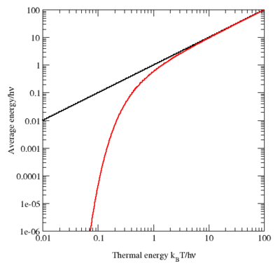
What’s the logic behind? Rayleigh’s Law gave the intensity for the various frequencies that are present as a function of (a) the frequency (of course!) and (b) the average energy of the oscillators, which is kT according to classical theory. Now, our assumption that an oscillator cannot take on just any energy value but that the energy levels are equally spaced, combined with Boltzmann’s Law, gives us a very different formula for the average energy: it’s a function of the temperature, but it’s a function of the fundamental frequency too! I copied the graph below from the Wikipedia article on the equipartition theorem. The black line is the classical value for the average energy as a function of the thermal energy. As you can see, it’s one and the same thing, really (look at the scales: they happen to be both logarithmic but that’s just to make them more ‘readable’). Its quantum-mechanical equivalent is the red curve. At higher temperatures, the two agree nearly perfectly, but at low temperatures (with low being defined as the range where kT << ħ·ω, written as h·ν in the graph), the quantum mechanical value decreases much more rapidly. [Note the energy is measured in units equivalent to h·ν: that’s a nice way to sort of ‘normalize’ things so as to compare them.]

So, without further ado, let’s take Rayleigh’s Law again and just substitute kT (i.e. the classical formula for the average energy) for the ‘quantum-mechanical’ formula for 〈E〉, i.e. ħω/[e^ħω/kT–1]. Adding the dω factor to emphasize we’re talking some continuous distribution here, we get the even grander result (Feynman calls it the first quantum-mechanical formula ever known or discussed):

So this function is the dashed I(ω) curve (I copied the graph below again): this curve does not ‘blow up’. The math behind the curve is the following: even for large ω, leading that ω³ factor in the numerator to ‘blow up’, we also have Euler’s number being raised to a tremendous power in the denominator. Therefore, the curves come down again, and so we don’t get those incredible amounts of UV light and x-rays.

So… That’s how Max Planck solved the problem and how he became the ‘reluctant father of quantum mechanics.’ The formula is not as simple as Rayleigh’s Law (we have a cubic function in the numerator, and an exponential in the denominator), but its advantage is that it’s correct. Indeed, when everything is said and done, indeed, we do want our formulas to describe something real, don’t we? 🙂

Let me conclude by looking at that ‘quantum-mechanical’ formula for the average energy once more:

〈E〉 = ħω/[e^ħω/kT–1]

It’s not a distribution function (the formula for I(ω) is the distribution function), but the –1 term in the denominator does tell us already we’re talking Bose-Einstein statistics. In my post on quantum statistics, I compared the three distribution functions. Let ‘s quickly look at them again:

• Maxwell-Boltzmann (for classical particles): f(E) = 1/[A·e^E/kT]
• Fermi-Dirac (for fermions): f(E) = 1/[Ae^E/kT + 1]
• Bose-Einstein (for bosons):  f(E) = 1/[Ae^E/kT − 1]

So here we simply substitute ħω for E, which makes sense, as the Planck-Einstein relation tells us that the energy of the particles involved is, indeed, equal to E = ħω . Below, you’ll find the graph of these three functions, first as a function of E, so that’s f(E), and then as a function of T, so that’s f(T) (or f(kT) if you want).

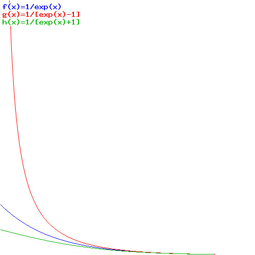
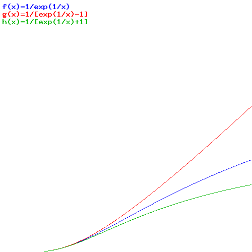
The first graph, for which E is the variable, is the more usual one. As for the interpretation, you can see what’s going on: bosonic particles (or bosons, I should say) will crowd the lower energy levels (the associated probabilities are much higher indeed), while for fermions, it’s the opposite: they don’t want to crowd together and, hence, the associated probabilities are much lower. So fermions will spread themselves over the various energy levels. The distribution for ‘classical’ particles is somewhere in the middle.

In that post of mine, I gave an actual example involving nine particles and the various patterns that are possible, so you can have a look there. Here I just want to note that the math behind is easy to understand when dropping the A (that’s just another normalization constant anyway) and re-writing the formulas as follows:

• Maxwell-Boltzmann (for classical particles): f(E) = e^−E/kT
• Fermi-Dirac (for fermions): f(E) = e^−E/kT/[1+e^−E/kT]
• Bose-Einstein (for bosons):  f(E) = e^−E/kT/[1−e^−E/kT]

Just use Feynman’s substitution x = e^−ħω/kT: the Bose-Einstein distribution then becomes 1/[1/x–1] = 1/[(1–x)/x] = x/(1–x). Now it’s easy to see that the denominator of the formula of both the Fermi-Dirac as well as the Bose-Einstein distribution will approach 1 (i.e. the ‘denominator’ of the Maxwell-Boltzmann formula) if e^−E/kT approaches zero, so that’s when E becomes larger and larger. Hence, for higher energy levels, the probability densities of the three functions approach each other indeed, as they should.

Now what’s the second graph about? Here we’re looking at one energy level only, but we let the temperature vary from 0 to infinity. The graph says that, at low temperature, the probabilities will also be more or less the same, and the three distributions only differ at higher temperatures. That makes sense too, of course!

Well… That says it all, I guess. I hope you enjoyed this post. As I’ve sort of concluded Volume I of Feynman’s Lectures with this, I’ll be silent for a while… […] Or so I think. 🙂

Some content on this page was disabled on June 16, 2020 as a result of a DMCA takedown notice from The California Institute of Technology. You can learn more about the DMCA here:

https://en.support.wordpress.com/copyright-and-the-dmca/
Some content on this page was disabled on June 16, 2020 as a result of a DMCA takedown notice from The California Institute of Technology. You can learn more about the DMCA here:

https://en.support.wordpress.com/copyright-and-the-dmca/
Some content on this page was disabled on June 16, 2020 as a result of a DMCA takedown notice from The California Institute of Technology. You can learn more about the DMCA here:

https://en.support.wordpress.com/copyright-and-the-dmca/
Some content on this page was disabled on June 16, 2020 as a result of a DMCA takedown notice from The California Institute of Technology. You can learn more about the DMCA here:

https://en.support.wordpress.com/copyright-and-the-dmca/