Systems with 2 spin-1/2 particles (I)

Pre-script (dated 26 June 2020): This post got mutilated by the removal of some material by the dark force. You should be able to follow the main story line, however. If anything, the lack of illustrations might actually help you to think things through for yourself. In any case, we now have different views on these concepts as part of our realist interpretation of quantum mechanics, so we recommend you read our recent papers instead of these old blog posts.

Original post:

I agree: this is probably the most boring title of a post ever. However, it should be interesting, as we’re going to apply what we’ve learned so far – i.e. the quantum-mechanical model of two-state systems – to a much more complicated problem—the solution of which can then be generalized to describe even more complicated situations.

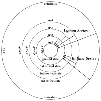
Two spin-1/2 particles? Let’s recall the most obvious example. In the ground state of a hydrogen atom (H), we have one electron that’s bound to one proton. The electron occupies the lowest energy state in its ground state, which – as Feynman shows in one of his first quantum-mechanical calculations – is equal to −13.6 eV. More or less, that is. 🙂  You’ll remember the reason for the minus sign: the electron has more energy when it’s unbound, which it releases as radiation when it joins an ionized hydrogen atom or, to put it simply, when a proton and an electron come together. In-between being bound and unbound, there are other discrete energy states – illustrated below – and we’ll learn how to describe the patterns of motion of the electron in each of those states soon enough.

Not in this post, however. 😦 In this post, we want to focus on the ground state only. Why? Just because. That’s today’s topic. 🙂 The proton and the electron can be in either of two spin states. As a result, the so-called ground state is not really a single definite-energy state. The spin states cause the so-called hyperfine structure in the energy levels: it splits them into several nearly equal energy levels, so that’s what referred to as hyperfine splitting.

[…] OK. Let’s go for it. As Feynman points out, the whole model is reduced to a set of four base states:

1. State 1: |++〉 = |1〉 (the electron and proton are both ‘up’)
2. State 2: |+−〉 = |2〉  (the electron is ‘up’ and the proton is ‘down’)
3. State 3: |−+〉 = |3〉  (the electron is ‘down’ and the proton is ‘up’)
4. State 4: |−−〉 = |4〉  (the electron and proton are both ‘down’)

The simplification is huge. As you know, the spin of electrically charged elementary particles is related to their motion in space, but so we don’t care about exact spatial relationships here: the direction of spin can be in any direction, but all that matters here is the relative orientation, and so all is simplified to some direction as defined by the proton and the electron itself. Full stop.

You know that the whole problem is to find the Hamiltonian coefficients, i.e. the energy matrix. Let me give them to you straight away. The energy levels involved are the following:

• E_I = E_II = E_III = A ≈ 9.23×10⁻⁶ eV
• E_IV = −3A ≈ 27.7×10⁻⁶ eV

So the difference in energy levels is measured in ten-millionths of an electron-volt and, hence, the hyperfine splitting is really hyper-fine. The question is: how do we get these values? So that is what this post is about. Let’s start by reminding ourselves of what we learned so far.

The Hamiltonian operator

We know that, in quantum mechanics, we describe any state in terms of the base states. In this particular case, we’d do so as follows:

|ψ〉 = |1〉C₁ + |2〉C₂ + |3〉C₃ +|4〉C₄ with C_i = 〈i|ψ〉

We refer to |ψ〉 as the spin state of the system, and so it’s determined by those four C_i amplitudes. Now, we know that those C_i amplitudes are functions of time, and they are, in turn, determined by the Hamiltonian matrix. To be precise, we find them by solving a set of linear differential equations that we referred to as Hamiltonian equations. To be precise, we’d describe the behavior of |ψ〉 in time by the following equation:

In case you forgot, the expression above is a short-hand for the following expression:

The index j would range over all base states and, therefore, this expression gives us everything we want: it really does describe the behavior, in time, of an N-state system. You’ll also remember that, when we’d use the Hamiltonian matrix in the way it’s used above (i.e. as an operator on a state), we’d put a little hat over it, so we defined the Hamiltonian operator as:

So far, so good—but this does not solve our problem: how do we find the Hamiltonian for this four-state system? What is it?

Well… There’s no one-size-fits-all answer to that: the analysis of two different two-state systems, like an ammonia molecule, or one spin-1/2 particle in a magnetic field, was different. Having said that, we did find we could generalize some of the solutions we’d find. For example, we’d write the Hamiltonian for a spin-1/2 particle, with a magnetic moment that’s assumed to be equal to μ, in a magnetic field B = (B_x, B_y, B_z) as:

In this equation, we’ve got a set of 4 two-by-two matrices (three so-called sigma matrices (σ_x, σ_y, σ_z), and then the unit matrix δ_ij = 1) which we referred to as the Pauli spin matrices, and which we wrote as:

You’ll remember that expression – which we further abbreviated, even more elegantly, to H = −μσ·B – covered all two-state systems involving a magnetic moment in a magnetic field. In fact, you’ll remember we could actually easily adapt the model to cover two-state systems in electric fields as well.

In short, these sigma matrices made our life very easy—as they covered a whole range of two-state models. So… Well… To make a long story short, what we want to do here is find some similar sigma matrices for four-state problems. So… Well… Let’s do that.

First, you should remind yourself of the fact that we could also use these sigma matrices as little operators themselves. To be specific, we’d let them ‘operate’ on the base states, and we’d find they’d do the following:

You need to read this carefully. What it says that the σ_z matrix, as an operator, acting on the ‘up’ base state, yields the same base state (i.e. ‘up’), and that the same operator, acting on the ‘down’ state, gives us the same but with a minus sign in front. Likewise, the σ_y matrix operating on the ‘up’ and ‘down’ states respectively, will give us i·|down〉 and −i·|up〉 respectively.

The trick to solve our problem here (i.e. our four-state system) is to apply those sigma matrices to the electron and the proton separately. Feynman introduces a new notation here by distinguishing the electron and proton sigma operators: the electron sigma operators (σ_x^e, σ_y^e, and σ_z^e) operate on the electron spin only, while – you guessed it – the proton sigma operator ((σ_x^p, σ_y^p, and σ_z^p) acts on the proton spin only. Applying it to the four states we’re looking at (i.e. |++〉, |+−〉, |−+〉 and |−−〉), we get the following bifurcation for our σ_x operator:

1. σ_x^e|++〉 = |−+〉
2. σ_x^e|+−〉 = |−−〉
3. σ_x^e|−+〉 = |++〉
4. σ_x^e|−−〉 = |+−〉
5. σ_x^p|++〉 = |+−〉
6. σ_x^p|+−〉 = |++〉
7. σ_x^p|−+〉 = |−−〉
8. σ_x^p|−−〉 = |−+〉

You get the idea. We had three operators acting on two states, i.e. 6 possibilities. Now we combine these three operators with two different particles, so we have six operators now, and we let them act on four possible system states, so we have 24 possibilities now. Now, we can, of course, let these operators act one after another. Check the following for example:

 σ_x^eσ_z^p|+−〉 = σ_x^e[σ_z^p|+−〉] = –σ_x^e|+−〉 = –|–−〉

[I now realize that I should have used the ↑ and ↓ symbols for the ‘up’ and ‘down’ states, as the minus sign is used to denote two very different things here, but… Well… So be it.]

Note that we only have nine possible σ_x^eσ_z^p-like combinations, because σ_x^eσ_z^p = σ_z^pσ_x^e, and then we have the 2×3 = six σ^e and σ^p operators themselves, so that makes for 15 new operators. [Note that the commutativity of these operators (σ_x^eσ_z^p = σ_z^pσ_x^e) is not some general property of quantum-mechanical operators.] If we include the unit operator (δ_ij = 1) – i.e. an operator that leaves all unchanged – we’ve got 16 in total. Now, we mentioned that we could write the Hamiltonian for a two-state system – i.e. a two-by-two matrix – as a linear combination of the four Pauli spin matrices. Likewise, one can demonstrate that the Hamiltonian for a four-state system can always be written as some linear combination of those sixteen ‘double-spin’ matrices. To be specific, we can write it as:

We should note a few things here. First, the E₀ constant is, of course, to be multiplied by the unit matrix, so we should actually write E₀δ_ij instead of E₀, but… Well… Quantum physicists always want to confuse you. 🙂 Second, the σ^eσ^p is like the σ·B notation: we can look at the σ_x^e, σ_y^e, σ_z^e and σ_x^p, σ_y^p, σ_z^p matrices as being the three components of two new (matrix) vectors, which we write as σ^e and σ^p respectively. Thirdly, and most importantly, you’ll want proof of that equation above. Well… I am sorry but I am going to refer you to Feynman here: he shows that the expression above “is the only thing that the Hamiltonian can be.” The proof is based on the fundamental symmetry of space. He also adds that space is symmetrical only so long as there is no external field. 🙂

Final question: what’s A? Well… Feynman is quite honest here as he says the following: “A can be calculated accurately once you understand the complete quantum theory of the hydrogen atom—which we so far do not. It has, in fact, been calculated to an accuracy of about 30 parts in one million. So, unlike the flip-flop constant A of the ammonia molecule, which couldn’t be calculated at all well by a theory, our constant A for the hydrogen can be calculated from a more detailed theory. But never mind, we will for our present purposes think of the A as a number which could be determined by experiment, and analyze the physics of the situation.”

So… Well… So far so good. We’ve got the Hamiltonian. That’s all we wanted, actually. But, now that we have come so far, let’s write it all out now.

Solving the equations

If that expression above is the Hamiltonian – and we assume it is, of course! – then our system of Hamiltonian equations can be written as:

[Note that we’ve switched to Newton’s ‘over-dot’ notation to denote time derivatives here.] Now, I could walk you through Feynman’s exposé but I guess you’ll trust the result. The equation above is equivalent to the following set of four equations:

We know that, because the Hamiltonian looks like this:

How do we know that? Well… Sorry: just check Feynman. 🙂 He just writes it all out. Now, we want to find those C_i functions. [When studying physics, the most important thing is to remember what it is that you’re trying to do. 🙂 ] Now, from my previous post (i.e. my post on the general solution for N-state systems), you’ll remember that those C_i functions should have the following functional form:

C_i(t) = a_i·e^{−i·(E/ħ)·t} 

If we substituting C_i(t) for that functional form in our set of Hamiltonian equations, we can cancel the exponentials so we get the following delightfully simple set of new equations:

The trivial solution, of course, is that all of the a_i coefficients are zero, but – as mentioned in my previous post – we’re looking for non-trivial solutions here. Well… From what you see above, it’s easy to appreciate that one non-trivial but simple solution is:

a₁ = 1 and a₂ = a₃ = a₄ = 0

So we’ve got one set of a_i coefficients here, and we’ll associate it with the first eigenvalue, or energy level, really—which we’ll denote as E_I. [I am just being consistent here with what I wrote in my previous post, which explained how general solutions to N-state systems look like.] So we find the following:

E_I = A

[Another thing you learn when studying physics is that the most amazing things are often summarized in super-terse equations, like this one here. 🙂 ]

But – Hey! Look at the symmetry between the first and last equation! 

We immediately get another simple – but non-trivial! – solution:

a₄ = 1 and a₁ = a₂ = a₃ = 0

We’ll associate the second energy level with that, so we write:

E_II = A

We’ve got two left. I’ll leave that to Feynman to solve:

Done! Four energy levels E_n (n = I, II, III, IV), and four associated energy state vectors – |n〉 – that describe their configuration (and which, as Feynman puts it, have the time dependence “factored out”). Perfect!

Now, we mentioned the experimental values:

• E_I = E_II = E_III = A ≈ 9.23×10⁻⁶ eV
• E_IV = −3A ≈ 27.7×10⁻⁶ eV

How can scientists measure these values? The theoretical analysis gives us the A and −3A values, but what about the empirical measurements? Well… We should find those values as the hydrogen atoms in state I, II or III should get rid of the energy by emitting some radiation. Now, the frequency of that radiation will give us the information we need, as illustrated below. The difference between E_I = E_II = E_III = A and E_IV = −3A (i.e. 4A) should correspond to the (angular) frequency of the radiation that’s being emitted or absorbed as atoms go from one energy state to the other. Now, hydrogen atoms do absorb and emit microwave radiation with a frequency that’s equal to 1,420,405,751.8 Hz. More or less, that is. 🙂 The standard error in the measurement is about two parts in 100 billion—and I am quoting some measurement done in the early 1960s here!]

Bingo! If f = ω/2π = (4A/ħ)/2π = 1,420,405,751.8 Hz, then A = f·2π·ħ/4 ≈ 9.23×10⁻⁶ eV.

So… Well… We’re done! I’ll see you tomorrow. 🙂 Tomorrow, we’re going to look at what happens when space is not symmetric, i.e. when we would have some external field! C u ! Cheers !

Some content on this page was disabled on June 16, 2020 as a result of a DMCA takedown notice from The California Institute of Technology. You can learn more about the DMCA here:

https://en.support.wordpress.com/copyright-and-the-dmca/
Some content on this page was disabled on June 16, 2020 as a result of a DMCA takedown notice from The California Institute of Technology. You can learn more about the DMCA here:

https://en.support.wordpress.com/copyright-and-the-dmca/
Some content on this page was disabled on June 20, 2020 as a result of a DMCA takedown notice from Michael A. Gottlieb, Rudolf Pfeiffer, and The California Institute of Technology. You can learn more about the DMCA here:

https://en.support.wordpress.com/copyright-and-the-dmca/
Some content on this page was disabled on June 20, 2020 as a result of a DMCA takedown notice from Michael A. Gottlieb, Rudolf Pfeiffer, and The California Institute of Technology. You can learn more about the DMCA here:

https://en.support.wordpress.com/copyright-and-the-dmca/
Some content on this page was disabled on June 20, 2020 as a result of a DMCA takedown notice from Michael A. Gottlieb, Rudolf Pfeiffer, and The California Institute of Technology. You can learn more about the DMCA here:

https://en.support.wordpress.com/copyright-and-the-dmca/
Some content on this page was disabled on June 20, 2020 as a result of a DMCA takedown notice from Michael A. Gottlieb, Rudolf Pfeiffer, and The California Institute of Technology. You can learn more about the DMCA here:

https://en.support.wordpress.com/copyright-and-the-dmca/