
Pre-script (dated 26 June 2020): This post got mutilated by the removal of some material by the dark force. You should be able to follow the main story line, however. If anything, the lack of illustrations might actually help you to think things through for yourself. In any case, we now have different views on these concepts as part of our realist interpretation of quantum mechanics, so we recommend you read our recent papers instead of these old blog posts.
Original post:
In our previous post, we noted the Hamiltonian for a simple system of two spin-1/2 particles—a proton and an electron (i.e. a hydrogen atom, in other words):
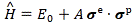
After noting that this Hamiltonian is “the only thing that it can be, by the symmetry of space, i.e. so long as there is no external field,” Feynman also notes the constant term (A) depends on the level we choose to measure energies from, so one might just as well take E0 = 0, in which case the formula reduces to H = Aσe·σp. Feynman analyzes this term as follows:
If there are two magnets near each other with magnetic moments μe and μp, the mutual energy will depend on μe·μp = |μe||μp|cosα = μeμpcosα — among other things. Now, the classical thing that we call μe or μp appears in quantum mechanics as μeσe and μpσp respectively (where μp is the magnetic moment of the proton, which is about 1000 times smaller than μe, and has the opposite sign). So the H = Aσe·σp equation says that the interaction energy is like the interaction between two magnets—only not quite, because the interaction of the two magnets depends on the radial distance between them. But the equation could be—and, in fact, is—some kind of an average interaction. The electron is moving all around inside the atom, and our Hamiltonian gives only the average interaction energy. All it says is that for a prescribed arrangement in space for the electron and proton there is an energy proportional to the cosine of the angle between the two magnetic moments, speaking classically. Such a classical qualitative picture may help you to understand where the H = Aσe·σp equation comes from.
That’s loud and clear, I guess. The next step is to introduce an external field. The formula for the Hamiltonian (we don’t distinguish between the matrix and the operator here) then becomes:
H = Aσe·σp − μeσe·B − μpσp·B
The first term is the term we already had. The second term is the energy the electron would have in the magnetic field if it were there alone. Likewise, the third term is the energy the proton would have in the magnetic field if it were there alone. When reading this, you should remember the following convention: classically, we write the energy U as U = −μ·B, because the energy is lowest when the moment is along the field. Hence, for positive particles, the magnetic moment is parallel to the spin, while for negative particles it’s opposite. In other words, μp is a positive number, while μe is negative. Feynman sums it all up as follows:
Classically, the energy of the electron and the proton together, would be the sum of the two, and that works also quantum mechanically. In a magnetic field, the energy of interaction due to the magnetic field is just the sum of the energy of interaction of the electron with the external field, and of the proton with the field—both expressed in terms of the sigma operators. In quantum mechanics these terms are not really the energies, but thinking of the classical formulas for the energy is a way of remembering the rules for writing down the Hamiltonian.
That’s also loud and clear. So now we need to solve those Hamiltonian equations once again. Feynman does so first assuming B is constant and in the z-direction. I’ll refer you to him for the nitty-gritty. The important thing is the results here:

He visualizes these – as a function of μB/A – as follows:
The illustration shows how the four energy levels have a different B-dependence:
- EI, EII, EIII start at (0, 1) but EI increases linearly with B—with slope μ, to be precise (cf. the EI = A + μB expression);
- In contrast, EII decreases linearly with B—again, with slope μ (cf. the EII = A − μB expression);
- We then have the EIII and EIV curves, which start out horizontally, to then curve and approach straight lines for large B, with slopes equal to μ’.
Oh—I realize I forget to define μ and μ’. Let me do that now: μ = −(μe+μp) and μ’ = −(μe−μp). And remember what we said above: μp is about 1000 times smaller than μe, and has opposite sign. OK. The point is: the magnetic field shifts the energy levels of our hydrogen atom. This is referred to as the Zeeman effect. Feynman describes it as follows:
The curves show the Zeeman splitting of the ground state of hydrogen. When there is no magnetic field, we get just one spectral line from the hyperfine structure of hydrogen. The transitions between state IV and any one of the others occurs with the absorption or emission of a photon whose (angular) frequency is 1/ħ times the energy difference 4A. [See my previous post for the calculation.] However, when the atom is in a magnetic field B, there are many more lines, and there can be transitions between any two of the four states. So if we have atoms in all four states, energy can be absorbed—or emitted—in any one of the six transitions shown by the vertical arrows in the illustration above.
The last question is: what makes the transitions go? Let me also quote Feynman’s answer to that:
The transitions will occur if you apply a small disturbing magnetic field that varies with time (in addition to the steady strong field B). It’s just as we saw for a varying electric field on the ammonia molecule. Only here, it is the magnetic field which couples with the magnetic moments and does the trick. But the theory follows through in the same way that we worked it out for the ammonia. The theory is the simplest if you take a perturbing magnetic field that rotates in the xy-plane—although any horizontal oscillating field will do. When you put in this perturbing field as an additional term in the Hamiltonian, you get solutions in which the amplitudes vary with time—as we found for the ammonia molecule. So you can calculate easily and accurately the probability of a transition from one state to another. And you find that it all agrees with experiment.
Alright! All loud and clear. 🙂
The magnetic quantum number
At very low magnetic fields, we still have the Zeeman splitting, but we can now approximate it as follows:
This simplified representation of things explains an older concept you may still see mentioned: the magnetic quantum number, which is usually denoted by m. Feynman’s explanation of it is quite straightforward, and so I’ll just copy it as is:
As he notes: the concept of the magnetic quantum number has nothing to do with new physics. It’s all just a matter of notation. 🙂
Well… This concludes our short study of four-state systems. On to the next! 🙂
Some content on this page was disabled on June 16, 2020 as a result of a DMCA takedown notice from The California Institute of Technology. You can learn more about the DMCA here:
https://wordpress.com/support/copyright-and-the-dmca/
Some content on this page was disabled on June 16, 2020 as a result of a DMCA takedown notice from The California Institute of Technology. You can learn more about the DMCA here:https://wordpress.com/support/copyright-and-the-dmca/
Some content on this page was disabled on June 16, 2020 as a result of a DMCA takedown notice from The California Institute of Technology. You can learn more about the DMCA here:https://wordpress.com/support/copyright-and-the-dmca/
Some content on this page was disabled on June 16, 2020 as a result of a DMCA takedown notice from The California Institute of Technology. You can learn more about the DMCA here:https://wordpress.com/support/copyright-and-the-dmca/
Some content on this page was disabled on June 16, 2020 as a result of a DMCA takedown notice from The California Institute of Technology. You can learn more about the DMCA here:
