
Pre-script (dated 26 June 2020): This post got mutilated by the removal of some material by the dark force. You should be able to follow the main story line, however. If anything, the lack of illustrations might actually help you to think things through for yourself. In any case, we now have different views on these concepts as part of our realist interpretation of quantum mechanics, so we recommend you read our recent papers instead of these old blog posts.
Original post:
I’ve said it a couple of times already: so far, we’ve only studied stuff that does not move in space. Hence, till now, time was the only variable in our wavefunctions. So now it’s time to… Well… Study stuff that does move in space. 🙂
Is that compatible with the title of this post? Solid-state physics? Solid-state stuff doesn’t move, does it? Well… No. But what we’re going to look at is how an electron travels through a solid crystal or, more generally, how an atomic excitation can travel through. In fact, what we’re really going to look at is how the wavefunction itself travels through space. However, that’s a rather bold statement, and so you should just read this post and judge for yourself. To be specific, we’re going to look at what happens in semiconductor material, like the silicon that’s used in microelectronic components like transistors and integrated circuits (ICs). You surely know the classical idea of that, which involves imagining an electron can be situated in a kind of ‘pit’ at one particular atom (or an electron hole, as it’s usually referred to), and it just moves from pit to pit. The Wikipedia article on it defines an electron hole as follows: an electron hole is the absence of an electron from a full valence band: the concept is used to conceptualize the interactions of the electrons within a nearly full system, i.e. a system which is missing just a few electrons. But here we’re going to forget about the classical picture. We’ll try to model it using the wavefunction concept. So how does that work? Feynman approaches it as follows.
If we look at a (one-dimensional) line of atoms – we can extend to a two- and three-dimensional analysis later – we may define an infinite number of base states for the extra electron that we think of as moving through the crystal. If the electron is with the n-th atom, then we’ll say it’s in a base state which we shall write as |n〉. Likewise, if it’s at atom n+1 or n−1, then we’ll associate that with base state |n+1〉 and |n−1〉 respectively. That’s what visualized below, and you should just along with the story here: don’t think classically, i.e. in terms of the electron is either here or, else, somewhere else. No. It’s got an amplitude to be anywhere. If you can’t take that… Well… I am sorry but that’s what QM is all about!

As usual, we write the amplitude for the electron to be in one of those states |n〉 as Cn(t) = 〈n|φ〉, and so we can the write the electron’s state at any point in time t by superposing all base states, so that’s the weighted sum of all base states, with the weights being equal to the associated amplitudes. So we write:
|φ〉 = ∑ |n〉Cn(t) = ∑ |n〉〈n|φ〉 over all n
Now we add some assumptions. One assumption is that an electron cannot directly jump to its next nearest neighbor: if it goes to the next nearest one, it will first have to go to nearest one. So two steps are needed to go from state |n−1〉 to state |n+1〉. This assumption simplifies the analysis: we can discuss more general cases later. To be specific, we’ll assume the amplitude to go from one base state to another, e.g. from |n〉 to |n+1〉, or |n−1〉 to state |n〉, is equal to i·A/ħ. You may wonder where this comes from, but it’s totally in line with equating our Hamiltonian non-diagonal elements to –A. Let me quickly insert a small digression here—for those who do really wonder where this comes from. 🙂
START OF DIGRESSION
Just check out those two-state systems we described, or that post of mine in which I explained why the following formulas are actually quite intuitive and easy to understand:
- U12(t + Δt, t) = − (i/ħ)·H12(t)·Δt = (i/ħ)·A·Δt and
- U21(t + Δt, t) = − (i/ħ)·H21(t)·Δt = (i/ħ)·A·Δt
More generally, you’ll remember that we wrote Uij(t + Δt, t) as:
Uij(t + Δt, t) = Uij(t, t) + Kij·Δt = δij(t, t) + Kij·Δt = δij(t, t) − (i/ħ)·Hij(t)·Δt
That looks monstrous but, frankly, what we have here is just a formula like this:
f(x+Δx) = f(x) + [df(x)/dt]·Δx
In case you didn’t notice, the formula is just the definition of the derivative if we write it as Δy/Δx = df(x)/dt for Δx → 0. Hence, the Kij coefficient in this formula is to be interpreted as a time derivative. Now, we re-wrote that Kij coefficient as the amplitude −(i/ħ)·Hij(t) and, therefore, that amplitude – i.e. the i·A/ħ factor (for i ≠ j) I introduced above – is to be interpreted as a time derivative. [Now that we’re here, let me quickly add that a time derivative gives the time rate of change of some quantity per unit time. So that i·A/ħ factor is also expressed per unit time.] We’d then just move the − (i/ħ) factor in that −(i/ħ)·Hij(t) coefficient to the other side to get the grand result we got for two-state systems, i.e. the Hamiltonian equations, which we could write in a number of ways, as shown below:
So… Well… That’s all there is to it, basically. Quantum math is not easy but, if anything, it is logical. You just have to get used to that imaginary unit (i) in front of stuff. That makes it always look very mysterious. 🙂 However, it should never scare you. You can just move it in or out of the differential operator, for example: i·df(x)/dt = d[i·f(x)]/dt. [Of course, i·f(x) ≠ f(i·x)!] So just think of i as a reminder that the number that follows it points in a different direction. To be precise: its angle with the other number is 90°. It doesn’t matter what we call those two numbers. The convention is to say that one is the real part of the wavefunction, while the other is the imaginary part but, frankly, in quantum math, both numbers are just as real. 🙂
END OF DIGRESSION
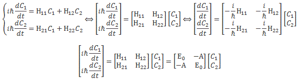
Yes. Let me get back to the lesson here. The assumption is that the Hamiltonian equations for our system here, i.e. the electron traveling from hole to hole, look like the following equation:
It’s really like those iħ·(dC1/dt) = E0C1 − AC2 and iħ·(dC2/dt) = − AC1 + E0C2 equations above, except that we’ve got three terms here:
- −(i/ħ)·E0 is the amplitude for the electron to just stay where it is, so we multiply that with the amplitude of the electron to be there at that time, i.e. the amplitude Cn(t), and bingo! That’s the first contribution to the time rate of change of the Cn amplitude (i.e. dCn/dt). [Note that all I brought that iħ factor in front to the other side: 1/(iħ) = −(i/ħ).] Of course, you also need to know what E0 is now: that’s just the (average) energy of our electron. So it’s really like the E0 of our ammonia molecule—or the average energy of any two-state system, really.
- −(i/ħ)·(−A) = i·A/ħ is the amplitude to go from one base state to another, i.e. from |n+1〉 to |n〉, for example. In fact, the second term models exactly that: i·A/ħ times the amplitude to be in state |n+1〉 is the second contribution to to the time rate of change of the Cn amplitude.
- Finally, the electron may also be in state |n−1〉 and go to |n〉 from there, so i·A/ħ times the amplitude to be in state |n−1〉 is yet another contribution to to the time rate of change of the Cn amplitude.
Now, we don’t want to think about what happens at the start and the end of our line of atoms, so we’ll just assume we’ve got an infinite number of them. As a result, we get an infinite number of equations, which Feynman summarizes as:
Holy cow! How do we solve that? We know that the general solution for those Cn amplitudes is likely to be some function like this:
Cn(t) = an·e−(i/ħ)·E·t
In case you wonder where this comes from, check my post on the general solution for N-state systems. If we substitute that trial solution in that iħ·(dCn/dt) = E0Cn − ACn+1 − ACn−1, we get:
Ean = E0an − Aan+1 − Aan−1
[Just do that derivative, and you’ll see the iħ can be scrapped. Also, the exponentials on both sides of the equation cancel each other out.] Now, that doesn’t look too bad, and we can also write it as (E − E0)·an = − A(an+1 + an−1 ), but… Well… What’s the next step? We’ve got an infinite number of coefficients an here, so we can’t use the usual methods to solve this set of equations. Feynman tries something completely different here. It looks weird but… Well… He gets a sensible result, so… Well… Let’s go for it.
He first writes these coefficients an as a function of a distance, which he defines as xn = xn−1 + b, with b the atomic spacing, i.e. the distance between two atoms (see the illustration). So now we write an = f(xn) = a(xn). Note that we don’t write an = fn(xn) = an(xn). No. It’s just one function f = a, not an infinite number of functions fn = an. Of course, once you see what comes of it, you’ll say: sure! The (complex) an coefficient in that function is the non-time-varying part of our function, and it’s about time we insert some part that’s varying in space and so… Well… Yes, of course! Our an coefficients don’t vary in time, so they must vary in space. Well… Yes. I guess so. 🙂 Our Ean = E0an − Aan+1 − Aan−1 equation becomes:
E·a(xn) = E0·a(xn) − A·a(xn+1) − A·a(xn+1) = E0·a(xn) − A·a(xn+b) − A·a(xn−b)
We can write this, once again, as (E − E0)·a(xn) = − A·[a(xn+b) + a(xn−b)]. Feynman notes this equation is like a differential equation, in the sense that it relates the value of some function (i.e. our a function, of course) at some point x to the values of the same function at nearby points, i.e. x ± b here. Frankly, I struggle a bit to see how it works exactly but Feynman now offers the following trial solution:
a(xn) = eikxn
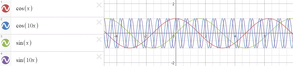
Huh? Why? And what’s k? Be patient. Just go along with this for a while. Let’s first do a graph. Think of xn as a nearly continuous variable representing position in space. We then know that this parameter k is then equal to the spatial frequency of our wavefunction: larger values for k give the wavefunction a higher density in space, as shown below.
In fact, I shouldn’t confuse you here, but you’ll surely think of the wavefunction you saw so many times already:
ψ(x, t) = a·e−i·[(E/ħ)·t − (p/ħ)∙x] = a·e−i·(ω·t − k∙x) = a·ei(k∙x−ω·t) = a·ei∙k∙x·e−i∙ω·t
This was the elementary wavefunction we’d associate with any particle, and so k would be equal to p/ħ, which is just the second of the two de Broglie relations: E = ħω and p = ħk (or, what amounts to the same: E = hf and λ = h/p). But you shouldn’t get confused. Not at this point. Or… Well… Not yet. 🙂
Let’s just take this proposed solution and plug it in. We get:
E·eikxn = E0·eikxn − A·eik(xn+b) − A·eik(xn−b) ⇔ E = E0 − A·eikb − A·e−ikb ⇔ E = E0 − 2A·cos(kb)
[In case you wonder what happens here: we just divide both sides by the common factor eikxn and then we also know that eiθ+e−iθ = 2·cosθ property.] So each k is associated with some energy E. In fact, to be precise, that E = E0 − 2A·cos(kb) function is a periodic function: it’s depicted below, and it reaches a maximum at k = ± π/b. [It’s easy to see why: E0 − 2A·cos(kb) reaches a maximum if cos(kb) = −1, i.e. if kb = ± π.]
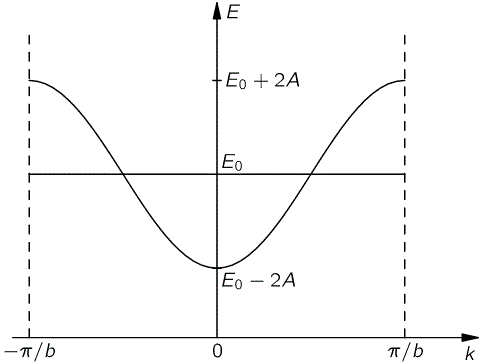
Of course, we still don’t really know what k or E are really supposed to represent, but think of it: it’s obvious that E can never be larger or smaller than E ± 2A, whatever the value of k. Note that, once again, it doesn’t matter if we used +A or −A in our equations: the energy band remains the same. And… Well… We’ve dropped the term now: the energy band of a semiconductor. That’s what it’s all about. What we’re saying here is that our electron, as it moves about, can have no other energies than the values in this band. Having said, that still doesn’t determine its energy: any energy level within that energy band is possible. So what does that mean? Hmm… Let’s take a break and not bother too much about k for the moment. Let’s look at our Cn(t) equations once more. We can now write them as:
Cn(t) = eikxn·e−(i/ħ)·E·t = eikxn·e−(i/ħ)·[E0 − 2A·cos(kb)]·t
You have enough experience now to sort of visualize what happens here. We can look at a certain xn value – read: a certain position in the lattice and watch, as time goes by, how the real and imaginary part of our little Cn wavefunction varies sinusoidally. We can also do it the other way around, and take a snapshot of the lattice at a certain point in time, and then we see how the amplitudes vary from point to point. That’s easy enough.
The thing is: we’re interested in probabilities in the end, and our wavefunction does not satisfy us in that regard: if we take the absolute square, its phase vanishes, and so we get the same probability everywhere! [Note that we didn’t normalize our wavefunctions here. It doesn’t matter. We can always do that later.] Now that’s not great. So what can we do about that? Now that’s where that k comes back in the game. Let’s have a look.
The effective mass of an electron
We’d like to find a solution which sort of ‘localizes’ our electron in space. Now, we know that we can do, in general, by superposing wavefunctions having different frequencies. There are a number of ways to go about, but the general idea is illustrated below.
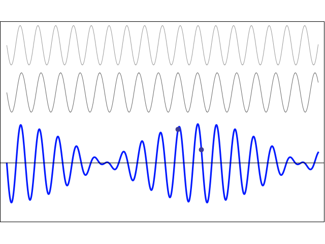
The first animation (for which credit must go to Wikipedia once more) is, obviously, the most sophisticated one. It shows how a new function – in red, and denoted by s6(x) – is constructed by summing six sine functions of different amplitudes and with harmonically related frequencies. This particular sum is referred to as a Fourier series, and the so-called Fourier transform, i.e. the S(f) function (in blue), depicts the six frequencies and their amplitudes.
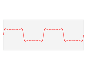
We’re more interested in the second animation here (for which credit goes to another nice site), which shows how a pattern of beats is created by just mixing two slightly different cosine waves. We want to do something similar here: we want to get a ‘wave packet‘ like the one below, which shows the real part only—but you can imagine the imaginary part 🙂 of course. [That’s exactly the same but with a phase shift, cf. the sine and cosine bit in Euler’s formula: eiθ = cosθ + i·sinθ.]
As you know, we must know make a distinction between the group velocity of the wave, and its phase velocity. That’s got to do with the dispersion relation, but we’re not going to get into the nitty-gritty here. Just remember that the group velocity corresponds to the classical velocity of our particle – so that must be the classical velocity of our electron here – and, equally important, also remember the following formula for that group velocity:
Let’s see how that plays out. The ω in this equation is equal to E/ħ = [E0 − 2A·cos(kb)]/ħ, so dω/dk = d[− (2A/ħ)·cos(kb)]/dk = (2Ab/ħ)·sin(kb). However, we’ll usually assume k is fairly small, so the variation of the amplitude from one xn to the other is fairly small. In that case, kb will be fairly small, and then we can use the so-called small angle approximation formula sin(ε) ≈ ε. [Note the reasoning here is a bit tricky, though, because – theoretically – k may vary between −π/b and +π/b and, hence, kb can take any value between −π and +π.] Using the small angle approximation, we get:
So we’ve got a quantum-mechanical calculation here that yields a classical velocity. Now, we can do something interesting now: we can calculate what is known as the effective mass of the electron, i.e. the mass that appears in the classical kinetic energy formula: K.E. = m·v2/2. Or in the classical momentum formula: p = m·v. So we can now write: K.E. = meff·v2/2 and p = meff·v. But… Well… The second de Broglie equation tells us that p = ħk, so we find that meff = ħk/v. Substituting v for what we’ve found above, gives us:
Unsurprisingly, we find that the value of meff is inversely proportional to A. It’s usually stated in units of the true mass of the electron, i.e. its mass in free space (me ≈ 9.11×10⁻³¹ kg) and, in these units, it’s usually in the range of 0.01 to 10. You’ll say: 0.01, i.e. one percent of its actual mass? Yes. An electron may travel more freely in matter than it does in free space. 🙂 That’s weird but… Well… Quantum mechanics is weird.
In any case, I’ll wrap this post up now. You’ ve got a nice model here. As Feynman puts it:
“We have now explained a remarkable mystery—how an electron in a crystal (like an extra electron put into germanium) can ride right through the crystal and flow perfectly freely even though it has to hit all the atoms. It does so by having its amplitudes going pip-pip-pip from one atom to the next, working its way through the crystal. That is how a solid can conduct electricity.”
Well… There you go. 🙂
Some content on this page was disabled on June 16, 2020 as a result of a DMCA takedown notice from The California Institute of Technology. You can learn more about the DMCA here:
https://wordpress.com/support/copyright-and-the-dmca/
Some content on this page was disabled on June 16, 2020 as a result of a DMCA takedown notice from The California Institute of Technology. You can learn more about the DMCA here:https://wordpress.com/support/copyright-and-the-dmca/
Some content on this page was disabled on June 16, 2020 as a result of a DMCA takedown notice from The California Institute of Technology. You can learn more about the DMCA here:https://wordpress.com/support/copyright-and-the-dmca/
Some content on this page was disabled on June 16, 2020 as a result of a DMCA takedown notice from The California Institute of Technology. You can learn more about the DMCA here:https://wordpress.com/support/copyright-and-the-dmca/
Some content on this page was disabled on June 16, 2020 as a result of a DMCA takedown notice from The California Institute of Technology. You can learn more about the DMCA here:https://wordpress.com/support/copyright-and-the-dmca/
Some content on this page was disabled on June 16, 2020 as a result of a DMCA takedown notice from The California Institute of Technology. You can learn more about the DMCA here:https://wordpress.com/support/copyright-and-the-dmca/
Some content on this page was disabled on June 16, 2020 as a result of a DMCA takedown notice from The California Institute of Technology. You can learn more about the DMCA here:

One thought on “Quantum math in solid-state physics”