
In our previous posts, we interpreted the elementary wavefunction ψ = a·e−i∙θ = a·cosθ − i·a·sinθ as a two-dimensional oscillation in spacetime. In addition to assuming the two directions of the oscillation were perpendicular to each other, we also assumed they were perpendicular to the direction of motion. While the first assumption is essential in our interpretation, the second assumption is solely based on an analogy with a circularly polarized electromagnetic wave. We also assumed the matter wave could be right-handed as well as left-handed (as illustrated below), and that these two physical possibilities corresponded to the angular momentum being equal to plus or minus ħ/2 respectively.


This allowed us to derive the Compton scattering radius of an elementary particle. Indeed, we interpreted the rotating vector as a resultant vector, which we get by adding the sine and cosine motions, which represent the real and imaginary components of our wavefunction. The energy of this two-dimensional oscillation is twice the energy of a one-dimensional oscillator and, therefore, equal to E = m·a2·ω2. Now, the angular frequency is given by ω = E/ħ and E must, obviously, also be equal to E = m·c2. Substitition and re-arranging the terms gives us the Compton scattering radius:
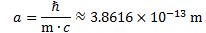
The value given above is the (reduced) Compton scattering radius for an electron. For a proton, we get a value of about 2.1×10⁻¹⁶ m, which is about 1/4 of the radius of a proton as measured in scattering experiments. Hence, for a proton, our formula does not give us the exact (i.e. experimentally verified) value but it does give us the correct order of magnitude—which is fine because we know a proton is not an elementary particle and, hence, the motion of its constituent parts (quarks) is… Well… It complicates the picture hugely.
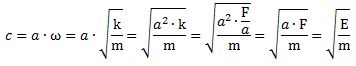
If we’d presume the electron charge would, effectively, be rotating about the center, then its tangential velocity is given by v = a·ω = [ħ·/(m·c)]·(E/ħ) = c, which is yet another wonderful implication of our hypothesis. Finally, the c = a·ω formula allowed us to interpret the speed of light as the resonant frequency of the fabric of space itself, as illustrated when re-writing this equality as follows:
This gave us a natural and forceful interpretation of Einstein’s mass-energy equivalence formula: the energy in the E = m·c2· equation is, effectively, a two-dimensional oscillation of mass.
However, while toying with this and other results (for example, we may derive a Poynting vector and show probabilities are, effectively, proportional to energy densities), I realize the plane of our two-dimensional oscillation cannot be perpendicular to the direction of motion of our particle. In fact, the direction of motion must lie in the same plane. This is a direct consequence of the direction of the angular momentum as measured by, for example, the Stern-Gerlach experiment. The basic idea here is illustrated below (credit for this illustration goes to another blogger on physics). As for the Stern-Gerlach experiment itself, let me refer you to a YouTube video from the Quantum Made Simple site.
 The point is: the direction of the angular momentum (and the magnetic moment) of an electron—or, to be precise, its component as measured in the direction of the (inhomogenous) magnetic field through which our electron is traveling—cannot be parallel to the direction of motion. On the contrary, it is perpendicular to the direction of motion. In other words, if we imagine our electron as some rotating disk or a flywheel, then it will actually comprise the direction of motion.
What are the implications? I am not sure. I will definitely need to review whatever I wrote about the de Broglie wavelength in previous posts. We will also need to look at those transformations of amplitudes once again. Finally, we will also need to relate this to the quantum-mechanical formulas for the angular momentum and the magnetic moment.
Post scriptum: As in previous posts, I need to mention one particularity of our model. When playing with those formulas, we contemplated two different formulas for the angular mass: one is the formula for a rotating mass (I = m·r2/2), and the other is the one for a rotating mass (I = m·r2). The only difference between the two is a 1/2 factor, but it turns out we need it to get a sensical result. For a rotating mass, the angular momentum is equal to the radius times the momentum, so that’s the radius times the mass times the velocity: L = m·v·r. [See also Feynman, Vol. II-34-2, in this regard)] Hence, for our model, we get L = m·v·r = m·c·a = m·c·ħ/(m·c) = ħ. Now, we know it’s equal to ±ħ/2, so we need that 1/2 factor in the formula.
Can we relate this 1/2 factor to the g-factor for the electron’s magnetic moment, which is (approximately) equal to 2? Maybe. We’d need to look at the formula for a rotating charged disk. That’s for a later post, however. It’s been enough for today, right? 🙂
I would just like to signal another interesting consequence of our model. If we would interpret the radius of our disk (a)—so that’s the Compton radius of our electron, as opposed to the Thomson radius—as the uncertainty in the position of our electron, then our L = m·v·r = m·c·a = p·a = ħ/2 formula as a very particular expression of the Uncertainty Principle: p·Δx= ħ/2. Isn’t that just plain nice? 🙂
Some content on this page was disabled on June 17, 2020 as a result of a DMCA takedown notice from Michael A. Gottlieb, Rudolf Pfeiffer, and The California Institute of Technology. You can learn more about the DMCA here:

One thought on “Electron spin and the geometry of the wavefunction”