Re-visiting the Uncertainty Principle

Pre-scriptum (dated 26 June 2020): This post suffered from the attack by the dark force. In any case, my views on the true nature of the concept of uncertainty in physics have evolved as part of my explorations of a more realist (classical) explanation of quantum mechanics. If you are reading this, then you are probably looking for not-to-difficult reading. In that case, I would suggest you read my re-write of Feynman’s introductory lecture to QM. If you want something shorter, you can also read my paper on what I believe to be the true Principles of Physics.

Original post:

Let me, just like Feynman did in his last lecture on quantum electrodynamics for Alix Mautner, discuss some loose ends. Unlike Feynman, I will not be able to tie them up. However, just describing them might be interesting and perhaps you, my imaginary reader, could actually help me with tying them up ! Let’s first re-visit the wave function for a photon by way of introduction.

The wave function for a photon

Let’s not complicate things from the start and, hence, let’s first analyze a nice Gaussian wave packet, such as the right-hand graph below: Ψ(x, t). It could be a de Broglie wave representing an electron but here we’ll assume the wave packet might actually represent a photon. [Of course, do remember we should actually show both the real as well as the imaginary part of this complex-valued wave function but we don’t want to clutter the illustration and so it’s only one of the two (cosine or sine). The ‘other’ part (sine or cosine) is just the same but with a phase shift. Indeed, remember that a complex number re^θ is equal to r(cosθ + isinθ), and the shape of the sine function is the same as the cosine function but it’s shifted to the left with π/2. So if we have one, we have the other. End of digression.]

The assumptions associated with this wonderful mathematical shape include the idea that the wave packet is a composite wave consisting of a large number of harmonic waves with wave numbers k₁, k₂_,k₃,… all lying around some mean value μ_k. That is what is shown in the left-hand graph. The mean value is actually noted as k-bar in the illustration above but because I can’t find a k-bar symbol among the ‘special characters’ in the text editor tool bar here, I’ll use the statistical symbols μ and σ to represent a mean value (μ) and some spread around it (σ). In any case, we have a pretty normal shape here, resembling the Gaussian distribution illustrated below.

These Gaussian distributions (also known as a density function) have outliers, but you will catch 95,4% of the observations within the μ ± 2σ interval, and 99.7% within the μ ± 3σ interval (that’s the so-called two- and three-sigma rule). Now, the shape of the left-hand graph of the first illustration, mapping the relation between k and A(k), is the same as this Gaussian density function, and if you would take a little ruler and measure the spread of k on the horizontal axis, you would find that the values for k are effectively spread over an interval that’s somewhat bigger than k-barplus or minus 2Δk. So let’s say 95,4% of the values of k lie in the interval [μ_k– 2Δk, μ_k+ 2Δk]. Hence, for all practical purposes, we can write that μ_k– 2Δk < k_n< μ_k+ 2Δk. In any case, we do not care too much about the rest because their contribution to the amplitude of the wave packet is minimal anyway, as we can see from that graph. Indeed, note that the A(k) values on the vertical axis of that graph do not represent the density of the k variable: there is only one wave number for each component wave, and so there’s no distribution or density function of k. These A(k) numbers represent the (maximum) amplitude of the component waves of our wave packet Ψ(x, t). In short, they are the values A(k) appearing in the summation formula for our composite wave, i.e. the wave packet:

I don’t want to dwell much more on the math here (I’ve done that in my other posts already): I just want you to get a general understanding of that ‘ideal’ wave packet possibly representing a photon above so you can follow the rest of my story. So we have a (theoretical) bunch of (component) waves with different wave numbers k_n, and the spread in these wave numbers – i.e. 2Δk, or let’s take 4Δk to make sure we catch (almost) all of them – determines the length of the wave packet Ψ, which is written here as 2Δx, or 4Δx if we’d want to include (most of) the tail ends as well. What else can we say about Ψ? Well… Maybe something about velocities and all that? OK.

To calculate velocities, we need both ω and k. Indeed, the phase velocity of a wave (v_p) is equal to v_p= ω/k. Now, the wave number k of the wave packet itself – i.e. the wave number of the oscillating ‘carrier wave’ so to say – should be equal to μ_kaccording to the article I took this illustration from. I should check that but, looking at that relationship between A(k) and k, I would not be surprised if the math behind is right. So we have the k for the wave packet itself (as opposed to the k’s of its components). However, I also need the angular frequency ω.

So what is that ω? Well… That will depend on all the ω’s associated with all the k’s, isn’t it? It does. But, as I explained in a previous post, the component waves do not necessarily have to travel all at the same speed and so the relationship between ω and k may not be simple. We would love that, of course, but Nature does what it wants. The only reasonable constraint we can impose on all those ω’s is that they should be some linear function of k. Indeed, if we do not want our wave packet to dissipate (or disperse or, to put it even more plainly, to disappear), then the so-called dispersion relation ω = ω(k) should be linear, so ω_nshould be equal to ω_n= ak_n+ b. What a and b? We don’t know. Random constants. But if the relationship is not linear, then the wave packet will disperse and it cannot possibly represent a particle – be it an electron or a photon.

I won’t go through the math all over again but in my Re-visiting the Matter Wave (I), I used the other de Broglie relationship (E = ħω) to show that – for matter waves that do not disperse – we will find that the phase velocity will equal c/β, with β = v/c, i.e. the ratio of the speed of our particle (v) and the speed of light (c). But, of course, photons travel at the speed of light and, therefore, everything becomes very simple and the phase velocity of the wave packet of our photon would equal the group velocity. In short, we have:

v_p= ω/k = v_g= ∂ω/∂k = c

Of course, I should add that the angular frequency of all component waves will also be equal to ω = ck, so all component waves of the wave packet representing a photon are supposed to travel at the speed of light! What an amazingly simple result!

It is. In order to illustrate what we have here – especially the elegance and simplicity of that wave packet for a photon – I’ve uploaded two gif files (see below). The first one could represent our ‘ideal’ photon: group and phase velocity (represented by the speed of the green and red dot respectively) are the same. Of course, our ‘ideal’ photon would only be one wave packet – not a bunch of them like here – but then you may want to think that the ‘beam’ below might represent a number of photons following each other in a regular procession.

The second animated gif below shows how phase and group velocity can differ. So that would be a (bunch of) wave packets representing a particle not traveling at the speed of light. The phase velocity here is faster than the group velocity (the red dot travels faster than the green dot). [One can actually also have a wave with positive group velocity and negative phase velocity – quite interesting ! – but so that would not represent a particle wave.] Again, a particle would be represented by one wave packet only (so that’s the space between two green dots only) but, again, you may want to think of this as representing electrons following each other in a very regular procession.

These illustrations (which I took, once again, from the online encyclopedia Wikipedia) are a wonderful pedagogic tool. I don’t know if it’s by coincidence but the group velocity of the second wave is actually somewhat slower than the first – so the photon versus electron comparison holds (electrons are supposed to move (much) slower). However, as for the phase velocities, they are the same for both waves and that would not reflect the results we found for matter waves. Indeed, you may or may not remember that we calculated superluminal speeds for the phase velocity of matter waves in that post I mentioned above (Re-visiting the Matter Wave): an electron traveling at a speed of 0.01c (1% of the speed of light) would be represented by a wave packet with a group velocity of 0.01c indeed, but its phase velocity would be 100 times the speed of light, i.e. 100c. [That being said, the second illustration may be interpreted as a little bit correct as the red dot does travel faster than the green dot, which – as I explained – is not necessarily always the case when looking at such composite waves (we can have slower or even negative speeds).]

Of course, I should once again repeat that we should not think that a photon or an electron is actually wriggling through space like this: the oscillation only represent the real or imaginary part of the complex-valued probability amplitude associated with our ‘ideal’ photon or our ‘ideal’ electron. That’s all. So this wave is an ‘oscillating complex number’, so to say, whose modulus we have to square to get the probability to actually find the photon (or electron) at some point x and some time t. However, the photon (or the electron) itself are just moving straight from left to right, with a speed matching the group velocity of their wave function.

Are they?

Well… No. Or, to be more precise: maybe. WHAT? Yes, that’s surely one ‘loose end’ worth mentioning! According to QED, photons also have an amplitude to travel faster or slower than light, and they are not necessarily moving in a straight line either. WHAT? Yes. That’s the complicated business I discussed in my previous post. As for the amplitudes to travel faster or slower than light, Feynman dealt with them very summarily. Indeed, you’ll remember the illustration below, which shows that the contributions of the amplitudes associated with slower or faster speed than light tend to nil because (a) their magnitude (or modulus) is smaller and (b) they point in the ‘wrong’ direction, i.e. not the direction of travel.

Still, these amplitudes are there and – Shock, horror ! – photons also have an amplitude to not travel in a straight line, especially when they are forced to travel through a narrow slit, or right next to some obstacle. That’s diffraction, described as “the apparent bending of waves around small obstacles and the spreading out of waves past small openings” in Wikipedia.

Diffraction is one of the many phenomena that Feynman deals with in his 1985 Alix G. Mautner Memorial Lectures. His explanation is easy: “not enough arrows” – read: not enough amplitudes to add. With few arrows, there are also few that cancel out indeed, and so the final arrow for the event is quite random, as shown in the illustrations below.

So… Not enough arrows… Feynman adds the following on this: “[For short distances] The nearby, nearly straight paths also make important contributions. So light doesn’t really travel only in a straight line; it “smells” the neighboring paths around it, and uses a small core of nearby space. In the same way, a mirror has to have enough size to reflect normally; if the mirror is too small for the core of neighboring paths, the light scatters in many directions, no matter where you put the mirror.” (QED, 1985, p. 54-56)

Not enough arrows… What does he mean by that? Not enough photons? No. Diffraction for photons works just the same as for electrons: even if the photons would go through the slit one by one, we would have diffraction (see my Revisiting the Matter Wave (II) post for a detailed discussion of the experiment). So even one photon is likely to take some random direction left or right after going through a slit, rather than to go straight. Not enough arrows means not enough amplitudes. But what amplitudes is he talking about?

These amplitudes have nothing to do with the wave function of our ideal photon we were discussing above: that’s the amplitude Ψ(x, t) of a photon to be at point x at point t. The amplitude Feynman is talking about is the amplitude of a photon to go from point A to B along one of the infinitely many possible paths it could take. As I explained in my previous post, we have to add all of these amplitudes to arrive at one big final arrow which, over longer distances, will usually be associated with a rather large probability that the photon will travel in a straight line and at the speed of light – which is why light seems to do at a macro-scale. 🙂

But back to that very succinct statement: not enough arrows. That’s obviously a very relative statement. Not enough as compared to what? What measurement scale are we talking about here? It’s obvious that the ‘scale’ of these arrows for electrons is different than for photons, because the 2012 diffraction experiment with electrons that I referred to used 50 nanometer slits (50×10⁻⁹ m), while one of the many experiments demonstrating light diffraction using pretty standard (red) laser light used slits of some 100 micrometer (that 100×10⁻⁶ m or – in units you are used to – 0.1 millimeter).

The key to the ‘scale’ here is the wavelength of these de Broglie waves: the slit needs to be ‘small enough’ as compared to these de Broglie wavelengths. For example, the width of the slit in the laser experiment corresponded to (roughly) 100 times the wavelength of the laser light, and the (de Broglie) wavelength of the electrons in that 2012 diffraction experiment was 50 picometer – that was actually a thousand times the electron wavelength – but it was OK enough to demonstrate diffraction. Much larger slits would not have done the trick. So, when it comes to light, we have diffraction at scales that do not involve nanotechnology, but when it comes to matter particles, we’re not talking micro but nano: that’s thousand times smaller.

The weird relation between energy and size

Let’s re-visit the Uncertainty Principle, even if Feynman says we don’t need that (we just need to do the amplitude math and we have it all). We wrote the uncertainty principle using the more scientific Kennard formulation: σ_xσ_p≥ ħ/2, in which the sigma symbol represents the standard deviation of position x and momentum p respectively. Now that’s confusing, you’ll say, because we were talking wave numbers, not momentum in the introduction above. Well… The wave number k of a de Broglie wave is, of course, related to the momentum p of the particle we’re looking at: p = ħk. Hence, a spread in the wave numbers amounts to a spread in the momentum really and, as I wanted to talk scales, let’s now check the dimensions.

The value for ħ is about 1×10^–34Joule·seconds (J·s) (it’s about 1.054571726(47)×10⁻³⁴ but let’s go with the gross approximation as for now). One J·s is the same as one kg·m²/s because 1 Joule is a shorthand for km kg·m²/s². It’s a rather large unit and you probably know that physicists prefer electronVolt·seconds (eV·s) because of that. However, even in expressed in eV·s the value for ħ comes out astronomically small: 6.58211928(15)×10⁻¹⁶ eV·s. In any case, because the J·s makes dimensions come out right, I’ll stick to it for a while. What does this incredible small factor of proportionality, both in the de Broglie relations as well in that Kennard formulation of the uncertainty principle, imply? How does it work out from a math point of view?

Well… It’s literally a quantum of measurement: even if Feynman says the uncertainty principle should just be seen “in its historical context”, and that “we don’t need it for adding arrows”, it is a consequence of the (related) position-space and momentum-space wave functions for a particle. In case you would doubt that, check it on Wikipedia: the author of the article on the uncertainty principle derives it from these two wave functions, which form a so-called Fourier transform pair. But so what does it say really?

Look at it. First, it says that we cannot know any of the two values exactly (exactly means 100%) because then we have a zero standard deviation for one or the other variable, and then the inequality makes no sense anymore: zero is obviously not greater or equal to 0.527286×10^–34J·s. However, the inequality with the value for ħ plugged in shows how close to zero we can get with our measurements. Let’s check it out.

Let’s use the assumption that two times the standard deviation (written as 2Δk or 2Δx on or above the two graphs in the very first illustration of this post) sort of captures the whole ‘range’ of the variable. It’s not a bad assumption: indeed, if Nature would follow normal distributions – and in our macro-world, that seems to be the case – then we’d capture 95.4 of them, so that’s good. Then we can re-write the uncertainty principle as:

Δx·σ_p≥ ħ or σ_x·Δp ≥ ħ

So that means we know x within some interval (or ‘range’ if you prefer that term) Δx or, else, we know p within some interval (or ‘range’ if you prefer that term) Δp. But we want to know both within some range, you’ll say. Of course. In that case, the uncertainty principle can be written as:

Δx·Δp≥ 2ħ

Huh? Why the factor 2? Well… Each of the two Δ ranges corresponds to 2σ (hence, σ_x= Δx/2 and σ_p= Δp/2), and so we have (1/2)Δx·(1/2)Δp≥ ħ/2. Note that if we would equate our Δ with 3σ to get 97.7% of the values, instead of 95.4% only, once again assuming that Nature distributes all relevant properties normally (not sure – especially in this case, because we are talking discrete quanta of action here – so Nature may want to cut off the ‘tail ends’!), then we’d get Δx·Δp≥ 4.5×ħ: the cost of extra precision soars! Also note that, if we would equate Δ with σ (the one-sigma rule corresponds to 68.3% of a normally distributed range of values), then we get yet another ‘version’ of the uncertainty principle: Δx·Δp≥ ħ/2. Pick and choose! And if we want to be purists, we should note that ħ is used when we express things in radians (such as the angular frequency for example: E = ħω), so we should actually use h when we are talking distance and (linear) momentum. The equation above then becomes Δx·Δp≥ h/π.

It doesn’t matter all that much. The point to note is that, if we express x and p in regular distance and momentum units (m and kg·m/s), then the unit for ħ (or h) is 1×10^–34. Now, we can sort of choose how to spread the uncertainty over x and p. If we spread it evenly, then we’ll measure both Δx and Δp in units of 1×10^–17 m and 1×10^–17kg·m/s. That’s small… but not that small. In fact, it is (more or less) imaginably small I’d say.

For example, a photon of a blue-violet light (let’s say a wavelength of around 660 nanometer) would have a momentum p = h/λ equal to some 1×10^–22 kg·m/s (just work it out using the values for h and λ). You would usually see this value measured in a unit that’s more appropriate to the atomic scale: 6.25 eV/c. [Converting momentum into energy using E = pc, and using the Joule-electronvolt conversion (1 eV ≈ 1.6×10^–19 J) will get you there.] Hence, units of 1×10^–17 m for momentum are a hundred thousand times the rather average momentum of our light photon. We can’t have that so let’s reduce the uncertainty related to the momentum to that 1×10^–22 kg·m/s scale. Then the uncertainty about position will be measured in units of 1×10^–12m. That’s the picometer scale in-between the nanometer (1×10^–9m) and the femtometer (1×10^–9m) scale. You’ll remember that this scale corresponds to the resolution of a (modern) electron microscope (50 pm). So can we see “uncertainty effects” ? Yes. I’ll come back to that.

However, before I discuss these, I need to make a little digression. Despite the sub-title I am using above, the uncertainties in distance and momentum we are discussing here are nowhere near to what is referred to as the Planck scale in physics: the Planck scale is at the other side of that Great Desert I mentioned: the Large Hadron Collider, which smashes particles with (average) energies of 4 tera-electronvolt (i.e. 4 trillion eV – all packed into one particle !) is probing stuff measuring at a scale of a thousandth of a femtometer (0.001×10^–12m), but we’re obviously at the limits of what’s technically possible, and so that’s where the Great Desert starts. The ‘other side’ of that Great Desert is the Planck scale: 10^–35m. Now, why is that some kind of theoretical limit? Why can’t we just continue to further cut these scales down? Just like Dedekind did when defining irrational numbers? We can surely get infinitely close to zero, can we? Well… No. The reasoning is quite complex (and I am not sure if I actually understand it – the way I should) but it is quite relevant to the topic here (the relation between energy and size), and it goes something like this:

In quantum mechanics, particles are considered to be point-like but they do take space, as evidenced from our discussion on slit widths: light will show diffraction at the micro-scale (10^–6m) but electrons will do that only at the nano-scale (10^–9m), so that’s a thousand times smaller. That’s related to their respective the de Broglie wavelength which, for electrons, is also a thousand times smaller than that of electrons. Now, the de Broglie wavelength is related to the energy and/or the momentum of these particles: E = hf and p = h/λ.
Higher energies correspond to smaller de Broglie wavelengths and, hence, are associated with particles of smaller size. To continue the example, the energy formula to be used in the E = hf relation for an electron – or any particle with rest mass – is the (relativistic) mass-energy equivalence relation: E = γm₀c², with γ the Lorentz factor, which depends on the velocity v of the particle. For example, electrons moving at more or less normal speeds (like in the 2012 experiment, or those used in an electron microscope) have typical energy levels of some 600 eV, and don’t think that’s a lot: the electrons from that cathode ray tube in the back of an old-fashioned TV which lighted up the screen so you could watch it, had energies in the 20,000 eV range. So, for electrons, we are talking energy levels a thousand or a hundred thousand higher than for your typical 2 to 10 eV photon.
Of course, I am not talking X or gamma rays here: hard X rays also have energies of 10 to 100 kilo-electronvolt, and gamma ray energies range from 1 million to 10 million eV (1-10 MeV). In any case, the point to note is ‘small’ particles must have high energies, and I am not only talking massless particles such as photons. Indeed, in my post End of the Road to Reality?, I discussed the scale of a proton and the scale of quarks: 1.7 and 0.7 femtometer respectively, which is smaller than the so-called classical electron radius. So we have (much) heavier particles here that are smaller? Indeed, the rest mass of the u and d quarks that make up a proton (uud) is 2.4 and 4.8 MeV/c² respectively, while the (theoretical) rest mass of an electron is 0.511 Mev/c²only, so that’s almost 20 times more: (2.4+2.4+4.8/0.5). Well… No. The rest mass of a proton is actually 1835 times the rest mass of an electron: the difference between the added rest masses of the quarks that make it up and the rest mass of the proton itself (938 MeV//c²) is the equivalent mass of the strong force that keeps the quarks together.
But let me not complicate things. Just note that there seems to be a strange relationship between the energy and the size of a particle: high-energy particles are supposed to be smaller, and vice versa: smaller particles are associated with higher energy levels. If we accept this as some kind of ‘factual reality’, then we may understand what the Planck scale is all about: : the energy levels associated with theoretical ‘particles’ of the above-mentioned Planck scale (i.e. particles with a size in the 10^–35m range) would have energy levels in the 10¹⁹GeV range. So what? Well… This amount of energy corresponds to an equivalent mass density of a black hole. So any ‘particle’ we’d associate with the Planck length would not make sense as a physical entity: it’s the scale where gravity takes over – everything.

Again: so what? Well… I don’t know. It’s just that this is entirely new territory, and it’s also not the topic of my post here. So let me just quote Wikipedia on this and then move on: “The fundamental limit for a photon’s energy is the Planck energy [that’s the 10¹⁹GeV which I mentioned above: to be precise, that ‘limit energy’ is said to be 1.22 × 10¹⁹GeV], for the reasons cited above [that ‘photon’ would not be ‘photon’ but a black hole, sucking up everything around it]. This makes the Planck scale a fascinating realm for speculation by theoretical physicists from various schools of thought. Is the Planck scale domain a seething mass of virtual black holes? Is it a fabric of unimaginably fine loops or a spin foam network? Is it interpenetrated by innumerable Calabi-Yau manifolds which connect our 3-dimensional universe with a higher-dimensional space? [That’s what’s string theory is about.] Perhaps our 3-D universe is ‘sitting’ on a ‘brane’ which separates it from a 2, 5, or 10-dimensional universe and this accounts for the apparent ‘weakness’ of gravity in ours. These approaches, among several others, are being considered to gain insight into Planck scale dynamics. This would allow physicists to create a unified description of all the fundamental forces. [That’s what’s these Grand Unification Theories (GUTs) are about.]

Hmm… I wish I could find some easy explanation of why higher energy means smaller size. I do note there’s an easy relationship between energy and momentum for massless particles traveling at the velocity of light (like photons): E = pc (or p = E/c), but – from what I write above – it is obvious that it’s the spread in momentum (and, therefore, in wave numbers) which determines how short or how long our wave train is, not the energy level as such. I guess I’ll just have to do some more research here and, hopefully, get back to you when I understand things better.

Re-visiting the Uncertainty Principle

You will probably have read countless accounts of the double-slit experiment, and so you will probably remember that these thought or actual experiments also try to watch the electrons as they pass the slits – with disastrous results: the interference pattern disappears. I copy Feynman’s own drawing from his 1965 Lecture on Quantum Behavior below: a light source is placed behind the ‘wall’, right between the two slits. Now, light (i.e. photons) gets scattered when it hits electrons and so now we should ‘see’ through which slit the electron is coming. Indeed, remember that we sent them through these slits one by one, and we still had interference – suggesting the ‘electron wave’ somehow goes through both slits at the same time, which can’t be true – because an electron is a particle.

However, let’s re-examine what happens exactly.

We can only detect all electrons if the light is high intensity, and high intensity does not mean higher energy photons but more photons. Indeed, if the light source is deem, then electrons might get through without being seen. So a high-intensity light source allows us to see all electrons but – as demonstrated not only in thought experiments but also in the laboratory – it destroys the interference pattern.
What if we use lower-energy photons, like infrared light with wavelengths of 10 to 100 microns instead of visible light? We can then use thermal imaging night vision goggles to ‘see’ the electrons. 🙂 And if that doesn’t work, we can use radiowaves (or perhaps radar!). The problem – as Feynman explains it – is that such low frequency light (associated with long wavelengths) only give a ‘big fuzzy flash’ when the light is scattered: “We can no longer tell which hole the electron went through! We just know it went somewhere!” At the same time, “the jolts given to the electron are now small enough so that we begin to see some interference effect again.” Indeed: “For wavelengths much longer than the separation between the two slits (when we have no chance at all of telling where the electron went), we find that the disturbance due to the light gets sufficiently small that we again get the interference curve P₁₂.” [P₁₂is the curve describing the original interference effect.]

Now, that would suggest that, when push comes to shove, the Uncertainty Principle only describes some indeterminacy in the so-called Compton scattering of a photon by an electron. This Compton scattering is illustrated below: it’s a more or less elastic collision between a photon and electron, in which momentum gets exchanged (especially the direction of the momentum) and – quite important – the wavelength of the scattered light is different from the incident radiation. Hence, the photon loses some energy to the electron and, because it will still travel at speed c, that means its wavelength must increase as prescribed by the λ = h/p de Broglie relation (with p = E/c for a photon). The change in the wavelength is called the Compton shift. and its formula is given in the illustration: it depends on the (rest) mass of the electron obviously and on the change in the direction of the momentum (of the photon – but that change in direction will obviously also be related to the recoil direction of the electron).

This is a very physical interpretation of the Uncertainty Principle, but it’s the one which the great Richard P. Feynman himself stuck to in 1965, i.e. when he wrote his famous Lectures on Physics at the height of his career. Let me quote his interpretation of the Uncertainty Principle in full indeed:

“It is impossible to design an apparatus to determine which hole the electron passes through, that will not at the same time disturb the electrons enough to destroy the interference pattern. If an apparatus is capable of determining which hole the electron goes through, it cannot be so delicate that it does not disturb the pattern in an essential way. No one has ever found (or even thought of) a way around this. So we must assume that it describes a basic characteristic of nature.”

That’s very mechanistic indeed, and it points to indeterminacy rather than ontological uncertainty. However, there’s weirder stuff than electrons being ‘disturbed’ in some kind of random way by the photons we use to detect them, with the randomness only being related to us not knowing at what time photons leave our light source, and what energy or momentum they have exactly. That’s just ‘indeterminacy’ indeed; not some fundamental ‘uncertainty’ about Nature.

We see such ‘weirder stuff’ in those mega- and now tera-electronvolt experiments in particle accelerators. In 1965, Feynman had access to the results of the high-energy positron-electron collisions being observed in the 3 km long Stanford Linear Accelerator (SLAC), which started working in 1961, but stuff like quarks and all that was discovered only in the late 1960s and early 1970s, so that’s after Feynman’s Lectures on Physics.So let me just mention a rather remarkable example of the Uncertainty Principle at work which Feynman quotes in his 1985 Alix G. Mautner Memorial Lectures on Quantum Electrodynamics.

In the Feynman diagram below, we see a photon disintegrating, at time t = T₃, into a positron and an electron. The positron (a positron is an electron with positive charge basically: it’s the electron’s anti-matter counterpart) meets another electron that ‘happens’ to be nearby and the annihilation results in (another) high-energy photon being emitted. While, as Feynman underlines, “this is a sequence of events which has been observed in the laboratory”, how is all this possible? We create matter – an electron and a positron both have considerable mass – out of nothing here ! [Well… OK – there’s a photon, so that’s some energy to work with…]

Feynman explains this weird observation without reference to the Uncertainty Principle. He just notes that “Every particle in Nature has an amplitude to move backwards in time, and therefore has an anti-particle.” And so that’s what this electron coming from the bottom-left corner does: it emits a photon and then the electron moves backwards in time. So, while we see a (very short-lived) positron moving forward, it’s actually an electron quickly traveling back in time according to Feynman! And, after a short while, it has had enough of going back in time, so then it absorbs a photon and continues in a slightly different direction. Hmm… If this does not sound fishy to you, it does to me.

The more standard explanation is in terms of the Uncertainty Principle applied to energy and time. Indeed, I mentioned that we have several pairs of conjugate variables in quantum mechanics: position and momentum are one such pair (related through the de Broglie relation p =ħk), but energy and time are another (related through the other de Broglie relation E = hf = ħω). While the ‘energy-time uncertainty principle’ – ΔE·Δt≥ ħ/2 – resembles the position-momentum relationship above, it is apparently used for ‘very short-lived products’ produced in high-energy collisions in accelerators only. I must assume the short-lived positron in the Feynman diagram is such an example: there is some kind of borrowing of energy (remember mass is equivalent to energy) against time, and then normalcy soon gets restored. Now THAT is something else than indeterminacy I’d say.

But so Feynman would say both interpretations are equivalent, because Nature doesn’t care about our interpretations.

What to say in conclusion? I don’t know. I obviously have some more work to do before I’ll be able to claim to understand the uncertainty principle – or quantum mechanics in general – somewhat. I think the next step is to solve my problem with the summary ‘not enough arrows’ explanation, which is – evidently – linked to the relation between energy and size of particles. That’s the one loose end I really need to tie up I feel ! I’ll keep you posted !

Some content on this page was disabled on June 16, 2020 as a result of a DMCA takedown notice from The California Institute of Technology. You can learn more about the DMCA here:

https://wordpress.com/support/copyright-and-the-dmca/
Some content on this page was disabled on June 20, 2020 as a result of a DMCA takedown notice from Michael A. Gottlieb, Rudolf Pfeiffer, and The California Institute of Technology. You can learn more about the DMCA here:

https://wordpress.com/support/copyright-and-the-dmca/

Light and matter

Pre-scriptum (dated 26 June 2020): This post does not seem to have suffered from the attack by the dark force. However, my views on the nature of light and matter have evolved as part of my explorations of a more realist (classical) explanation of quantum mechanics. If you are reading this, then you are probably looking for not-to-difficult reading. In that case, I would suggest you read my re-write of Feynman’s introductory lecture to QM. If you want something shorter, you can also read my paper on what I believe to be the true Principles of Physics.

Original post:

In my previous post, I discussed the de Broglie wave of a photon. It’s usually referred to as ‘the’ wave function (or the psi function) but, as I explained, for every psi – i.e. the position-space wave function Ψ(x ,t) – there is also a phi – i.e. the momentum-space wave function Φ(p, t).

In that post, I also compared it – without much formalism – to the de Broglie wave of ‘matter particles’. Indeed, in physics, we look at ‘stuff’ as being made of particles and, while the taxonomy of the particle zoo of the Standard Model of physics is rather complicated, one ‘taxonomic’ principle stands out: particles are either matter particles (known as fermions) or force carriers (known as bosons). It’s a strict separation: either/or. No split personalities.

A quick overview before we start…

Wikipedia’s overview of particles in the Standard Model (including the latest addition: the Higgs boson) illustrates this fundamental dichotomy in nature: we have the matter particles (quarks and leptons) on one side, and the bosons (i.e. the force carriers) on the other side.

Standard_Model_of_Elementary_Particles

Don’t be put off by my remark on the particle zoo: it’s a term coined in the 1960s, when the situation was quite confusing indeed (like more than 400 ‘particles’). However, the picture is quite orderly now. In fact, the Standard Model put an end to the discovery of ‘new’ particles, and it’s been stable since the 1970s, as experiments confirmed the reality of quarks. Indeed, all resistance to Gell-Man’s quarks and his flavor and color concepts – which are just words to describe new types of ‘charge’ – similar to electric charge but with more variety), ended when experiments by Stanford’s Linear Accelerator Laboratory (SLAC) in November 1974 confirmed the existence of the (second-generation and, hence, heavy and unstable) ‘charm’ quark (again, the names suggest some frivolity but it’s serious physical research).

As for the Higgs boson, its existence of the Higgs boson had also been predicted, since 1964 to be precise, but it took fifty years to confirm it experimentally because only something like the Large Hadron Collider could produce the required energy to find it in these particle smashing experiments – a rather crude way of analyzing matter, you may think, but so be it. [In case you harbor doubts on the Higgs particle, please note that, while CERN is the first to admit further confirmation is needed, the Nobel Prize Committee apparently found the evidence ‘evidence enough’ to finally award Higgs and others a Nobel Prize for their ‘discovery’ fifty years ago – and, as you know, the Nobel Prize committee members are usually rather conservative in their judgment. So you would have to come up with a rather complex conspiracy theory to deny its existence.]

Also note that the particle zoo is actually less complicated than it looks at first sight: the (composite) particles that are stable in our world – this world – consist of three quarks only: a proton consists of two up quarks and one down quark and, hence, is written as uud., and a neutron is two down quarks and one up quark: udd. Hence, for all practical purposes (i.e. for our discussion how light interacts with matter), only the so-called first generation of matter-particles – so that’s the first column in the overview above – are relevant.

All the particles in the second and third column are unstable. That being said, they survive long enough – a muon disintegrates after 2.2 millionths of a second (on average) – to deserve the ‘particle’ title, as opposed to a ‘resonance’, whose lifetime can be as short as a billionth of a trillionth of a second – but we’ve gone through these numbers before and so I won’t repeat that here. Why do we need them? Well… We don’t, but they are a by-product of our world view (i.e. the Standard Model) and, for some reason, we find everything what this Standard Model says should exist, even if most of the stuff (all second- and third-generation matter particles, and all these resonances, vanish rather quickly – but so that also seems to be consistent with the model). [As for a possible fourth (or higher) generation, Feynman didn’t exclude it when he wrote his 1985 Lectures on quantum electrodynamics, but, checking on Wikipedia, I find the following: “According to the results of the statistical analysis by researchers from CERN and the Humboldt University of Berlin, the existence of further fermions can be excluded with a probability of 99.99999% (5.3 sigma).” If you want to know why… Well… Read the rest of the Wikipedia article. It’s got to do with the Higgs particle.]

As for the (first-generation) neutrino in the table – the only one which you may not be familiar with – these are very spooky things but – I don’t want to scare you – relatively high-energy neutrinos are going through your and my my body, right now and here, at a rate of some hundred trillion per second. They are produced by stars (stars are huge nuclear fusion reactors, remember?), and also as a by-product of these high-energy collisions in particle accelerators of course. But they are very hard to detect: the first trace of their existence was found in 1956 only – 26 years after their existence had been postulated: the fact that Wolfgang Pauli proposed their existence in 1930 to explain how beta decay could conserve energy, momentum and spin (angular momentum) demonstrates not only the genius but also the confidence of these early theoretical quantum physicists. Most neutrinos passing through Earth are produced by our Sun. Now they are being analyzed more routinely. The largest neutrino detector on Earth is called IceCube. It sits on the South Pole – or under it, as it’s suspended under the Antarctic ice, and it regularly captures high-energy neutrinos in the range of 1 to 10 TeV.

Let me – to conclude this introduction – just quickly list and explain the bosons (i.e the force carriers) in the table above:

1. Of all of the bosons, the photon (i.e. the topic of this post), is the most straightforward: there is only type of photon, even if it comes in different possible states of polarization.

[…]

I should probably do a quick note on polarization here – even if all of the stuff that follows will make abstraction of it. Indeed, the discussion on photons that follows (largely adapted from Feynman’s 1985 Lectures on Quantum Electrodynamics) assumes that there is no such thing as polarization – because it would make everything even more complicated. The concept of polarization (linear, circular or elliptical) has a direct physical interpretation in classical mechanics (i.e. light as an electromagnetic wave). In quantum mechanics, however, polarization becomes a so-called qubit (quantum bit): leaving aside so-called virtual photons (these are short-range disturbances going between a proton and an electron in an atom – effectively mediating the electromagnetic force between them), the property of polarization comes in two basis states (0 and 1, or left and right), but these two basis states can be superposed. In ket notation: if ¦0〉 and ¦1〉 are the basis states, then any linear combination α·¦0〉 + ß·¦1〉 is also a valid state provided│α│²+ │β│²= 1, in line with the need to get probabilities that add up to one.

In case you wonder why I am introducing these kets, there is no reason for it, except that I will be introducing some other tools in this post – such as Feynman diagrams – and so that’s all. In order to wrap this up, I need to note that kets are used in conjunction with bras. So we have a bra-ket notation: the ket gives the starting condition, and the bra – denoted as 〈 ¦ – gives the final condition. They are combined in statements such as 〈 particle arrives at x¦particle leaves from s〉 or – in short – 〈 x¦s〉 and, while x and s would have some real-number value, 〈 x¦s〉 would denote the (complex-valued) probability amplitude associated wit the event consisting of these two conditions (i.e the starting and final condition).

But don’t worry about it. This digression is just what it is: a digression. Oh… Just make a mental note that the so-called virtual photons (the mediators that are supposed to keep the electron in touch with the proton) have four possible states of polarization – instead of two. They are related to the four directions of space (x, y and z) and time (t). 🙂

2. Gluons, the exchange particles for the strong force, are more complicated: they come in eight so-called colors. In practice, one should think of these colors as different charges, but so we have more elementary charges in this case than just plus or minus one (±1) – as we have for the electric charge. So it’s just another type of qubit in quantum mechanics.

[Note that the so-called elementary ±1 values for electric charge are not really elementary: it’s –1/3 (for the down quark, and for the second- and third-generation strange and bottom quarks as well) and +2/3 (for the up quark as well as for the second- and third-generation charm and top quarks). That being said, electric charge takes two values only, and the ±1 value is easily found from a linear combination of the –1/3 and +2/3 values.]

3. Z and W bosons carry the so-called weak force, aka as Fermi’s interaction: they explain how one type of quark can change into another, thereby explaining phenomena such as beta decay. Beta decay explains why carbon-14 will, after a very long time (as compared to the ‘unstable’ particles mentioned above), spontaneously decay into nitrogen-14. Indeed, carbon-12 is the (very) stable isotope, while carbon-14 has a life-time of 5,730 ± 40 years ‘only’ (so one can’t call carbon-12 ‘unstable’: perhaps ‘less stable’ will do) and, hence, measuring how much carbon-14 is left in some organic substance allows us to date it (that’s what (radio)carbon-dating is about). As for the name, a beta particle can refer to an electron or a positron, so we can have β^–decay (e.g. the above-mentioned carbon-14 decay) as well as β⁺decay (e.g. magnesium-23 into sodium-23). There’s also alpha and gamma decay but that involves different things.

As you can see from the table, W^±and Z⁰bosons are very heavy (157,000 and 178,000 times heavier than a electron!), and W^±carry the (positive or negative) electric charge. So why don’t we see them? Well… They are so short-lived that we can only see a tiny decay width, just a very tiny little trace, so they resemble resonances in experiments. That’s also the reason why we see little or nothing of the weak force in real-life: the force-carrying particles mediating this force don’t get anywhere.

4. Finally, as mentioned above, the Higgs particle – and, hence, of the associated Higgs field – had been predicted since 1964 already but its existence was only (tentatively) experimentally confirmed last year. The Higgs field gives fermions, and also the W and Z bosons, mass (but not photons and gluons), and – as mentioned above – that’s why the weak force has such short range as compared to the electromagnetic and strong forces. Note, however, that the Higgs particle does actually not explain the gravitational force, so it’s not the (theoretical) graviton and there is no quantum field theory for the gravitational force as yet. Just Google it and you’ll quickly find out why: there’s theoretical as well as practical (experimental) reasons for that.

The Higgs field stands out from the other force fields because it’s a scalar field (as opposed to a vector field). However, I have no idea how this so-called Higgs mechanism (i.e. the interaction with matter particles (i.e. with the quarks and leptons, but not directly with neutrinos it would seem from the diagram below), with W and Z bosons, and with itself – but not with the massless photons and gluons) actually works. But then I still have a very long way to go on this Road to Reality.

In any case… The topic of this post is to discuss light and its interaction with matter – not the weak or strong force, nor the Higgs field.

Let’s go for it.

Amplitudes, probabilities and observable properties

Being born a boson or a fermion makes a big difference. That being said, both fermions and bosons are wavicles described by a complex-valued psi function, colloquially known as the wave function. To be precise, there will be several wave functions, and the square of their modulus (sorry for the jargon) will give you the probability of some observable property having a value in some relevant range, usually denoted by Δ. [I also explained (in my post on Bose and Fermi) how the rules for combining amplitudes differ for bosons versus fermions, and how that explains why they are what they are: matter particles occupy space, while photons not only can but also like to crowd together in, for example, a powerful laser beam. I’ll come back on that.]

For all practical purposes, relevant usually means ‘small enough to be meaningful’. For example, we may want to calculate the probability of detecting an electron in some tiny spacetime interval (Δx, Δt). [Again, ‘tiny’ in this context means small enough to be relevant: if we are looking at a hydrogen atom (whose size is a few nanometer), then Δx is likely to be a cube or a sphere with an edge or a radius of a few picometer only (a picometer is a thousandth of a nanometer, so it’s a millionth of a millionth of a meter); and, noting that the electron’s speed is approximately 2200 km per second… Well… I will let you calculate a relevant Δt. :-)]

If we want to do that, then we will need to square the modulus of the corresponding wave function Ψ(x, t). To be precise, we will have to do a summation of all the values │Ψ(x, t)│²over the interval and, because x and t are real (and, hence, continuous) numbers, that means doing some integral (because an integral is the continuous version of a sum).

But that’s only one example of an observable property: position. There are others. For example, we may not be interested in the particle’s exact position but only in its momentum or energy. Well, we have another wave function for that: the momentum wave function Φ(x ,t). In fact, if you looked at my previous posts, you’ll remember the two are related because they are conjugate variables: Fourier transforms duals of one another. A less formal way of expressing that is to refer to the uncertainty principle. But this is not the time to repeat things.

The bottom line is that all particles travel through spacetime with a backpack full of complex-valued wave functions. We don’t know who and where these particles are exactly, and so we can’t talk to them – but we can e-mail God and He’ll send us the wave function that we need to calculate some probability we are interested in because we want to check – in all kinds of experiments designed to fool them – if it matches with reality.

As mentioned above, I highlighted the main difference between bosons and fermions in my Bose and Fermi post, so I won’t repeat that here. Just note that, when it comes to working with those probability amplitudes (that’s just another word for these psi and phi functions), it makes a huge difference: fermions and bosons interact very differently. Bosons are party particles: they like to crowd and will always welcome an extra one. Fermions, on the other hand, will exclude each other: that’s why there’s something referred to as the Fermi exclusion principle in quantum mechanics. That’s why fermions make matter (matter needs space) and bosons are force carriers (they’ll just call friends to help when the load gets heavier).

Light versus matter: Quantum Electrodynamics

OK. Let’s get down to business. This post is about light, or about light-matter interaction. Indeed, in my previous post (on Light), I promised to say something about the amplitude of a photon to go from point A to B (because – as I wrote in my previous post – that’s more ‘relevant’, when it comes to explaining stuff, than the amplitude of a photon to actually be at point x at time t), and so that’s what I will do now.

In his 1985 Lectures on Quantum Electrodynamics (which are lectures for the lay audience), Feynman writes the amplitude of a photon to go from point A to B as P(A to B) – and the P stands for photon obviously, not for probability. [I am tired of repeating that you need to square the modulus of an amplitude to get a probability but – here you are – I have said it once more.] That’s in line with the other fundamental wave function in quantum electrodynamics (QED): the amplitude of an electron to go from A to B, which is written as E(A to B). [You got it: E just stands for electron, not for our electric field vector.]

I also talked about the third fundamental amplitude in my previous post: the amplitude of an electron to absorb or emit a photon. So let’s have a look at these three. As Feynman says: ““Out of these three amplitudes, we can make the whole world, aside from what goes on in nuclei, and gravitation, as always!”

Well… Thank you, Mr Feynman: I’ve always wanted to understand the World (especially if you made it).

The photon-electron coupling constant j

Let’s start with the last of those three amplitudes (or wave functions): the amplitude of an electron to absorb or emit a photon. Indeed, absorbing or emitting makes no difference: we have the same complex number for both. It’s a constant – denoted by j (for junction number) – equal to –0.1 (a bit less actually but it’s good enough as an approximation in the context of this blog).

Huh? Minus 0.1? That’s not a complex number, is it? It is. Real numbers are complex numbers too: –0.1 is 0.1e^iπin polar coordinates. As Feynman puts it: it’s “a shrink to about one-tenth, and half a turn.” The ‘shrink’ is the 0.1 magnitude of this vector (or arrow), and the ‘half-turn’ is the angle of π (i.e. 180 degrees). He obviously refers to multiplying (no adding here) j with other amplitudes, e.g. P(A, C) and E(B, C) if the coupling is to happen at or near C. And, as you’ll remember, multiplying complex numbers amounts to adding their phases, and multiplying their modulus (so that’s adding the angles and multiplying lengths).

Let’s introduce a Feynman diagram at this point – drawn by Feynman himself – which shows three possible ways of two electrons exchanging a photon. We actually have two couplings here, and so the combined amplitude will involve two j‘s. In fact, if we label the starting point of the two lines representing our electrons as 1 and 2 respectively, and their end points as 3 and 4, then the amplitude for these events will be given by:

E(1 to 5)·j·E(5 to 3)·E(2 to 6)·j·E(6 to 3)

As for how that j factor works, please do read the caption of the illustration below: the same j describes both emission as well as absorption. It’s just that we have both an emission as well as an as absorption here, so we have a j²factor here, which is less than 0.1·0.1 = 0.01. At this point, it’s worth noting that it’s obvious that the amplitudes we’re talking about here – i.e. for one possible way of an exchange like the one below happening – are very tiny. They only become significant when we add many of these amplitudes, which – as explained below – is what has to happen: one has to consider all possible paths, calculate the amplitudes for them (through multiplication), and then add all these amplitudes, to then – finally – square the modulus of the combined ‘arrow’ (or amplitude) to get some probability of something actually happening. [Again, that’s the best we can do: calculate probabilities that correspond to experimentally measured occurrences. We cannot predict anything in the classical sense of the word.]

A Feynman diagram is not just some sketchy drawing. For example, we have to care about scales: the distance and time units are equivalent (so distance would be measured in light-seconds or, else, time would be measured in units equivalent to the time needed for light to travel one meter). Hence, particles traveling through time (and space) – from the bottom of the graph to the top – will usually not be traveling at an angle of more than 45 degrees (as measured from the time axis) but, from the graph above, it is clear that photons do. [Note that electrons moving through spacetime are represented by plain straight lines, while photons are represented by wavy lines. It’s just a matter of convention.]

More importantly, a Feynman diagram is a pictorial device showing what needs to be calculated and how. Indeed, with all the complexities involved, it is easy to lose track of what should be added and what should be multiplied, especially when it comes to much more complicated situations like the one described above (e.g. making sense of a scattering event). So, while the coupling constant j (aka as the ‘charge’ of a particle – but it’s obviously not the electric charge) is just a number, calculating an actual E(A to B) amplitudes is not easy – not only because there are many different possible routes (paths) but because (almost) anything can happen. Let’s have a closer look at it.

E(A to B)

As Feynman explains in his 1985 QED Lectures: “E(A to B) can be represented as a giant sum of a lot of different ways an electron can go from point A to B in spacetime: the electron can take a ‘one-hop flight’, going directly from point A to B; it could take a ‘two-hop flight’, stopping at an intermediate point C; it could take a ‘three-hop flight’ stopping at points D and E, and so on.”

Fortunately, the calculation re-uses known values: the amplitude for each ‘hop’ – from C to D, for example – is P(F to G) – so that’s the amplitude of a photon (!) to go from F to G – even if we are talking an electron here. But there’s a difference: we also have to multiply the amplitudes for each ‘hop’ with the amplitude for each ‘stop’, and that’s represented by another number – not j but n². So we have an infinite series of terms for E(A to B): P(A to B) + P(A to C)·n²·P(C to B) + P(A to D)·n²·P(D to E)·n²·P(E to B) + … for all possible intermediate points C, D, E, and so on, as per the illustration below.

You’ll immediately ask: what’s the value of n? It’s quite important to know it, because we want to know how big these n², n⁴etcetera terms are. I’ll be honest: I have not come to terms with that yet. According to Feynman (QED, p. 125), it is the ‘rest mass’ of an ‘ideal’ electron: an ‘ideal’ electron is an electron that doesn’t know Feynman’s amplitude theory and just goes from point to point in spacetime using only the direct path. 🙂 Hence, it’s not a probability amplitude like j: a proper probability amplitude will always have a modulus less than 1, and so when we see exponential terms like j², j⁴,… we know we should not be all that worried – because these sort of vanish (go to zero) for sufficiently large exponents. For E(A to B), we do not have such vanishing terms. I will not dwell on this right here, but I promise to discuss it in the Post Scriptum of this post. The frightening possibility is that n might be a number larger than one.

[As we’re freewheeling a bit anyway here, just a quick note on conventions: I should not be writing j in bold-face, because it’s a (complex- or real-valued) number and symbols representing numbers are usually not written in bold-face: vectors are written in bold-face. So, while you can look at a complex number as a vector, well… It’s just one of these inconsistencies I guess. The problem with using bold-face letters to represent complex numbers (like amplitudes) is that they suggest that the ‘dot’ in a product (e.g. j·j) is an actual dot project (aka as a scalar product or an inner product) of two vectors. That’s not the case. We’re multiplying complex numbers here, and so we’re just using the standard definition of a product of complex numbers. This subtlety probably explains why Feynman prefers to write the above product as P(A to B) + P(A to C)*n²*P(C to B) + P(A to D)*n²*P(D to E)*n²*P(E to B) + … But then I find that using that asterisk to represent multiplication is a bit funny (although it’s a pretty common thing in complex math) and so I am not using it. Just be aware that a dot in a product may not always mean the same type of multiplication: multiplying complex numbers and multiplying vectors is not the same. […] And I won’t write j in bold-face anymore.]

P(A to B)

Regardless of the value for n, it’s obvious we need a functional form for P(A to B), because that’s the other thing (other than n) that we need to calculate E(A to B). So what’s the amplitude of a photon to go from point A to B?

Well… The function describing P(A to B) is obviously some wave function – so that’s a complex-valued function of x and t. It’s referred to as a (Feynman) propagator: a propagator function gives the probability amplitude for a particle to travel from one place to another in a given time, or to travel with a certain energy and momentum. [So our function for E(A to B) will be a propagator as well.] You can check out the details on it on Wikipedia. Indeed, I could insert the formula here, but believe me if I say it would only confuse you. The points to note is that:

The propagator is also derived from the wave equation describing the system, so that’s some kind of differential equation which incorporates the relevant rules and constraints that apply to the system. For electrons, that’s the Schrödinger equation I presented in my previous post. For photons… Well… As I mentioned in my previous post, there is ‘something similar’ for photons – there must be – but I have not seen anything that’s equally ‘simple’ as the Schrödinger equation for photons. [I have Googled a bit but it’s obvious we’re talking pretty advanced quantum mechanics here – so it’s not the QM-101 course that I am currently trying to make sense of.]
The most important thing (in this context at least) is that the key variable in this propagator (i.e. the Feynman propagator for the photon) is I: that spacetime interval which I mentioned in my previous post already:

I = Δr²– Δt² = (z₂– z₁)²+ (y₂– y₁)²+ (x₂– x₁)²– (t₂– t₁)²

In this equation, we need to measure the time and spatial distance between two points in spacetime in equivalent units (these ‘points’ are usually referred to as four-vectors), so we’d use light-seconds for the unit of distance or, for the unit of time, the time it takes for light to travel one meter. [If we don’t want to transform time or distance scales, then we have to write I as I = c²Δt² – Δr².] Now, there are three types of intervals:

For time-like intervals, we have a negative value for I, so Δt²> Δr². For two events separated by a time-like interval, enough time passes between them so there could be a cause–effect relationship between the two events. In a Feynman diagram, the angle between the time axis and the line between the two events will be less than 45 degrees from the vertical axis. The traveling electrons in the Feynman diagrams above are an example.
For space-like intervals, we have a positive value for I, so Δt²< Δr². Events separated by space-like intervals cannot possibly be causally connected. The photons traveling between point 5 and 6 in the first Feynman diagram are an example, but then photons do have amplitudes to travel faster than light.
Finally, for light-like intervals, I = 0, or Δt²= Δr². The points connected by the 45-degree lines in the illustration below (which Feynman uses to introduce his Feynman diagrams) are an example of points connected by light-like intervals.

[Note that we are using the so-called space-like convention (+++–) here for I. There’s also a time-like convention, i.e. with +––– as signs: I = Δt² – Δr²so just check when you would consult other sources on this (which I recommend) and if you’d feel I am not getting the signs right.]

Now, what’s the relevance of this? To calculate P(A to B), we have to add the amplitudes for all possible paths that the photon can take, and not in space, but in spacetime. So we should add all these vectors (or ‘arrows’ as Feynman calls them) – an infinite number of them really. In the meanwhile, you know it amounts to adding complex numbers, and that infinite sums are done by doing integrals, but let’s take a step back: how are vectors added?

Well…That’s easy, you’ll say… It’s the parallelogram rule… Well… Yes. And no. Let me take a step back here to show how adding a whole range of similar amplitudes works.

The illustration below shows a bunch of photons – real or imagined – from a source above a water surface (the sun for example), all taking different paths to arrive at a detector under the water (let’s say some fish looking at the sky from under the water). In this case, we make abstraction of all the photons leaving at different times and so we only look at a bunch that’s leaving at the same point in time. In other words, their stopwatches will be synchronized (i.e. there is no phase shift term in the phase of their wave function) – let’s say at 12 o’clock when they leave the source. [If you think this simplification is not acceptable, well… Think again.]

When these stopwatches hit the retina of our poor fish’s eye (I feel we should put a detector there, instead of a fish), they will stop, and the hand of each stopwatch represents an amplitude: it has a modulus (its length) – which is assumed to be the same because all paths are equally likely (this is one of the first principles of QED) – but their direction is very different. However, by now we are quite familiar with these operations: we add all the ‘arrows’ indeed (or vectors or amplitudes or complex numbers or whatever you want to call them) and get one big final arrow, shown at the bottom – just above the caption. Look at it very carefully.

If you look at the so-called contribution made by each of the individual arrows, you can see that it’s the arrows associated with the path of least time and the paths immediately left and right of it that make the biggest contribution to the final arrow. Why? Because these stopwatches arrive around the same time and, hence, their hands point more or less in the same direction. It doesn’t matter what direction – as long as it’s more or less the same.

[As for the calculation of the path of least time, that has to do with the fact that light is slowed down in water. Feynman shows why in his 1985 Lectures on QED, but I cannot possibly copy the whole book here ! The principle is illustrated below.]

So, where are we? This digressions go on and on, don’t they? Let’s go back to the main story: we want to calculate P(A to B), remember?

As mentioned above, one of the first principles in QED is that all paths – in spacetime – are equally likely. So we need to add amplitudes for every possible path in spacetime using that Feynman propagator function. You can imagine that will be some kind of integral which you’ll never want to solve. Fortunately, Feynman’s disciples have done that for you already. The results is quite predictable: the grand result is that light has a tendency to travel in straight lines and at the speed of light.

WHAT!? Did Feynman get a Nobel prize for trivial stuff like that?

Yes. The math involved in adding amplitudes over all possible paths not only in space but also in time uses the so-called path integral formulation of quantum mechanics and so that’s got Feynman’s signature on it, and that’s the main reason why he got this award – together with Julian Schwinger and Sin-Itiro Tomonaga: both much less well known than Feynman, but so they shared the burden. Don’t complain about it. Just take a look at the ‘mechanics’ of it.

We already mentioned that the propagator has the spacetime interval I in its denominator. Now, the way it works is that, for values of I equal or close to zero, so the paths that are associated with light-like intervals, our propagator function will yield large contributions in the ‘same’ direction (wherever that direction is), but for the spacetime intervals that are very much time- or space-like, the magnitude of our amplitude will be smaller and – worse – our arrow will point in the ‘wrong’ direction. In short, the arrows associated with the time- and space-like intervals don’t add up to much, especially over longer distances. [When distances are short, there are (relatively) few arrows to add, and so the probability distribution will be flatter: in short, the likelihood of having the actual photon travel faster or slower than speed is higher.]

Conclusion

Does this make sense? I am not sure, but I did what I promised to do. I told you how P(A to B) gets calculated; and from the formula for E(A to B), it is obvious that we can then also calculate E(A to B) provided we have a value for n. However, that value n is determined experimentally, just like the value of j, in order to ensure this amplitude theory yields probabilities that match the probabilities we observe in all kinds of crazy experiments that try to prove or disprove the theory; and then we can use these three amplitude formulas “to make the whole world”, as Feynman calls it, except the stuff that goes on inside of nuclei (because that’s the domain of the weak and strong nuclear force) and gravitation, for which we have a law (Newton’s Law) but no real ‘explanation’. [Now, you may wonder if this QED explanation of light is really all that good, but Mr Feynman thinks it is, and so I have no reason to doubt that – especially because there’s surely not anything more convincing lying around as far as I know.]

So what remains to be told? Lots of things, even within the realm of expertise of quantum electrodynamics. Indeed, Feynman applies the basics as described above to a number of real-life phenomena – quite interesting, all of it ! – but, once again, it’s not my goal to copy all of his Lectures here. [I am only hoping to offer some good summaries of key points in some attempt to convince myself that I am getting some of it at least.] And then there is the strong force, and the weak force, and the Higgs field, and so and so on. But that’s all very strange and new territory which I haven’t even started to explore. I’ll keep you posted as I am making my way towards it.

Post scriptum: On the values of j and n

In this post, I promised I would write something about how we can find j and n because I realize it would just amount to copy three of four pages out of that book I mentioned above, and which inspired most of this post. Let me just say something more about that remarkable book, and then quote a few lines on what the author of that book – the great Mr Feynman ! – thinks of the math behind calculating these two constants (the coupling constant j, and the ‘rest mass’ of an ‘ideal’ electron). Now, before I do that, I should repeat that he actually invented that math (it makes use of a mathematical approximation method called perturbation theory) and that he got a Nobel Prize for it.

First, about the book. Feynman’s 1985 Lectures on Quantum Electrodynamics are not like his 1965 Lectures on Physics. The Lectures on Physics are proper courses for undergraduate and even graduate students in physics. This little 1985 book on QED is just a series of four lectures for a lay audience, conceived in honor of Alix G. Mautner. She was a friend of Mr Feynman’s who died a few years before he gave and wrote these ‘lectures’ on QED. She had a degree in English literature and would ask Mr Feynman regularly to explain quantum mechanics and quantum electrodynamics in a way she would understand. While they had known each other for about 22 years, he had apparently never taken enough time to do so, as he writes in his Introduction to these Alix G. Mautner Memorial Lectures: “So here are the lectures I really [should have] prepared for Alix, but unfortunately I can’t tell them to her directly, now.”

The great Richard Phillips Feynman himself died only three years later, in February 1988 – not of one but two rare forms of cancer. He was only 69 years old when he died. I don’t know if he was aware of the cancer(s) that would kill him, but I find his fourth and last lecture in the book, Loose Ends, just fascinating. Here we have a brilliant mind deprecating the math that earned him a Nobel Prize and without which the Standard Model would be unintelligible. I won’t try to paraphrase him. Let me just quote him. [If you want to check the quotes, the relevant pages are page 125 to 131):

The math behind calculating these constants] is a “dippy process” and “having to resort to such hocus-pocus has prevented us from proving that the theory of quantum electrodynamics is mathematically self-consistent“. He adds: “It’s surprising that the theory still hasn’t been proved self-consistent one way or the other by now; I suspect that renormalization [“the shell game that we play to find n and j” as he calls it] is not mathematically legitimate.” […] Now, Mr Feynman writes this about quantum electrodynamics, not about “the rest of physics” (and so that’s quantum chromodynamics (QCD) – the theory of the strong interactions – and quantum flavordynamics (QFD) – the theory of weak interactions) which, he adds, “has not been checked anywhere near as well as electrodynamics.”

That’s a pretty damning statement, isn’t it? In one of my other posts (see: The End of the Road to Reality?), I explore these comments a bit. However, I have to admit I feel I really need to get back to math in order to appreciate these remarks. I’ve written way too much about physics anyway now (as opposed to the my first dozen of posts – which were much more math-oriented). So I’ll just have a look at some more stuff indeed (such as perturbation theory), and then I’ll get back blogging. Indeed, I’ve written like 20 posts or so in a few months only – so I guess I should shut up for while now !

In the meanwhile, you’re more than welcome to comment of course !

Light

Original post:

I started the two previous posts attempting to justify why we need all these mathematical formulas to understand stuff: because otherwise we just keep on repeating very simplistic but nonsensical things such as ‘matter behaves (sometimes) like light’, ‘light behaves (sometimes) like matter’ or, combining both, ‘light and matter behave like wavicles’. Indeed: what does ‘like‘ mean? Like the same but different? 🙂 However, I have not said much about light so far.

Light and matter are two very different things. For matter, we have quantum mechanics. For light, we have quantum electrodynamics (QED). However, QED is not only a quantum theory about light: as Feynman pointed out in his little but exquisite 1985 book on quantum electrodynamics (QED: The Strange Theory of Light and Matter), it is first and foremost a theory about how light interacts with matter. However, let’s limit ourselves here to light.

In classical physics, light is an electromagnetic wave: it just travels on and on and on because of that wonderful interaction between electric and magnetic fields. A changing electric field induces a magnetic field, the changing magnetic field then induces an electric field, and then the changing electric field induces a magnetic field, and… Well, you got the idea: it goes on and on and on. This wonderful machinery is summarized in Maxwell’s equations – and most beautifully so in the so-called Heaviside form of these equations, which assume a charge-free vacuum space (so there are no other charges lying around exerting a force on the electromagnetic wave or the (charged) particle whom’s behavior we want to study) and they also make abstraction of other complications such as electric currents (so there are no moving charges going around either).

I reproduced Heaviside’s Maxwell equations below as well as an animated gif which is supposed to illustrate the dynamics explained above. [In case you wonder who’s Heaviside? Well… Check it out: he was quite a character.] The animation is not all that great but OK enough. And don’t worry if you don’t understand the equations – just note the following:

The electric and magnetic field E and B are represented by perpendicular oscillating vectors.
The first and third equation (∇·E = 0 and ∇·B = 0) state that there are no static or moving charges around and, hence, they do not have any impact on (the flux of) E and B.
The second and fourth equation are the ones that are essential. Note the time derivatives (∂/∂t): E and B oscillate and perpetuate each other by inducing new circulation of B and E.

The constants μ and ε in the fourth equation are the so-called permeability (μ) and permittivity (ε) of the medium, and μ₀ and ε₀ are the values for these constants in a vacuum space. Now, it is interesting to note that με equals 1/c², so a changing electric field only produces a tiny change in the circulation of the magnetic field. That’s got something to do with magnetism being a ‘relativistic’ effect but I won’t explore that here – except for noting that the final Lorentz force on a (charged) particle F = q(E + v×B) will be the same regardless of the reference frame (moving or inertial): the reference frame will determine the mixture of E and B fields, but there is only one combined force on a charged particle in the end, regardless of the reference frame (inertial or moving at whatever speed – relativistic (i.e. close to c) or not). [The forces F, E and B on a moving (charged) particle are shown below the animation of the electromagnetic wave.] In other words, Maxwell’s equations are compatible with both special as well as general relativity. In fact, Einstein observed that these equations ensure that electromagnetic waves always travel at speed c (to use his own words: “Light is always propagated in empty space with a definite velocity c which is independent of the state of motion of the emitting body.”) and it’s this observation that led him to develop his special relativity theory.

The other interesting thing to note is that there is energy in these oscillating fields and, hence, in the electromagnetic wave. Hence, if the wave hits an impenetrable barrier, such as a paper sheet, it exerts pressure on it – known as radiation pressure. [By the way, did you ever wonder why a light beam can travel through glass but not through paper? Check it out!] A very oft-quoted example is the following: if the effects of the sun’s radiation pressure on the Viking spacecraft had been ignored, the spacecraft would have missed its Mars orbit by about 15,000 kilometers. Another common example is more science fiction-oriented: the (theoretical) possibility of space ships using huge sails driven by sunlight (paper sails obviously – one should not use transparent plastic for that).

I am mentioning radiation pressure because, although it is not that difficult to explain radiation pressure using classical electromagnetism (i.e. light as waves), the explanation provided by the ‘particle model’ of light is much more straightforward and, hence, a good starting point to discuss the particle nature of light:

Electromagnetic radiation is quantized in particles called photons. We know that because of Max Planck’s work on black body radiation, which led to Planck’s relation: E = hν. Photons are bona fide particles in the so-called Standard Model of physics: they are defined as bosons with spin 1, but zero rest mass and no electric charge (as opposed to W bosons). They are denoted by the letter or symbol γ (gamma), so that’s the same symbol that’s used to denote gamma rays. [Gamma rays are high-energy electromagnetic radiation (i.e. ‘light’) that have a very definite particle character. Indeed, because of their very short wavelength – less than 10 picometer (10×10^{–12 m}) and high energy (hundreds of KeV – as opposed to visible light, which has a wavelength between 380 and 750 nanometer (380-750×10^{–9 m}) and typical energy of 2 to 3 eV only (so a few hundred thousand times less), they are capable of penetrating through thick layers of concrete, and the human body – where they might damage intracellular bodies and create cancer (lead is a more efficient barrier obviously: a shield of a few centimeter of lead will stop most of them. In case you are not sure about the relation between energy and penetration depth, see the Post Scriptum.]
Although photons are considered to have zero rest mass, they have energy and, hence, an equivalent relativistic mass (m = E/c²) and, therefore, also momentum. Indeed, energy and momentum are related through the following (relativistic) formula: E = (p²c²+ m₀²c⁴)^1/2(the non-relativistic version is simply E = p²/2m₀ but – quite obviously – an approximation that cannot be used in this case – if only because the denominator would be zero). This simplifies to E = pc or p = E/c in this case. This basically says that the energy (E) and the momentum (p) of a photon are proportional, with c – the velocity of the wave – as the factor of proportionality.
The generation of radiation pressure can then be directly related to the momentum property of photons, as shown in the diagram below – which shows how radiation force could – perhaps – propel a space sailing ship. [Nice idea, but I’d rather bet on nuclear-thermal rocket technology.]

I said in my introduction to this post that light and matter are two very different things. They are, and the logic connecting matter waves and electromagnetic radiation is not straightforward – if there is any. Let’s look at the two equations that are supposed to relate the two – the de Broglie relation and the Planck relation:

The de Broglie relation E = hf assigns a de Broglie frequency (i.e. the frequency of a complex-valued probability amplitude function) to a particle with mass m through the mass-energy equivalence relation E = mc². However, the concept of a matter wave is rather complicated (if you don’t think so: read the two previous posts): matter waves have little – if anything – in common with electromagnetic waves. Feynman calls electromagnetic waves ‘real’ waves (just like water waves, or sound waves, or whatever other wave) as opposed to… Well – he does stop short of calling matter waves unreal but it’s obvious they look ‘less real’ than ‘real waves’. Indeed, these complex-valued psi functions (Ψ) – for which we have to square the modulus to get the probability of something happening in space and time, or to measure the likely value of some observable property of the system – are obviously ‘something else’! [I tried to convey their ‘reality’ as well as I could in my previous post, but I am not sure I did a good job – not all really.]
The Planck relation E = hν relates the energy of a photon – the so-called quantum of light (das Lichtquant as Einstein called it in 1905 – the term ‘photon’ was coined some 20 years later it is said) – to the frequency of the electromagnetic wave of which it is part. [That Greek symbol (ν) – it’s the letter nu (the ‘v’ in Greek is amalgamated with the ‘b’) – is quite confusing: it’s not the v for velocity.]

So, while the Planck relation (which goes back to 1905) obviously inspired Louis de Broglie (who introduced his theory on electron waves some 20 years later – in his PhD thesis of 1924 to be precise), their equations look the same but are different – and that’s probably the main reason why we keep two different symbols – f and ν – for the two frequencies.

Photons and electrons are obviously very different particles as well. Just to state the obvious:

Photons have zero rest mass, travel at the speed of light, have no electric charge, are bosons, and so on and so on, and so they behave differently (see, for example, my post on Bose and Fermi, which explains why one cannot make proton beam lasers). [As for the boson qualification, bosons are force carriers: photons in particular mediate (or carry) the electromagnetic force.]
Electrons do not weigh much and, hence, can attain speeds close to light (but it requires tremendous amounts of energy to accelerate them very near c) but so they do have some mass, they have electric charge (photons are electrically neutral), and they are fermions – which means they’re an entirely different ‘beast’ so to say when it comes to combining their probability amplitudes (so that’s why they’ll never get together in some kind of electron laser beam either – just like protons or neutrons – as I explain in my post on Bose and Fermi indeed).

That being said, there’s some connection of course (and that’s what’s being explored in QED):

Accelerating electric charges cause electromagnetic radiation (so moving charges (the negatively charged electrons) cause the electromagnetic field oscillations, but it’s the (neutral) photons that carry it).
Electrons absorb and emit photons as they gain/lose energy when going from one energy level to the other.
Most important of all, individual photons – just like electrons – also have a probability amplitude function – so that’s a de Broglie or matter wave function if you prefer that term.

That means photons can also be described in terms of some kind of complex wave packet, just like that electron I kept analyzing in my previous posts – until I (and surely you) got tired of it. That means we’re presented with the same type of mathematics. For starters, we cannot be happy with assigning a unique frequency to our (complex-valued) de Broglie wave, because that would – once again – mean that we have no clue whatsoever where our photon actually is. So, while the shape of the wave function below might well describe the E and B of a bona fide electromagnetic wave, it cannot describe the (real or imaginary) part of the probability amplitude of the photons we would associate with that wave.

So that doesn’t work. We’re back at analyzing wave packets – and, by now, you know how complicated that can be: I am sure you don’t want me to mention Fourier transforms again! So let’s turn to Feynman once again – the greatest of all (physics) teachers – to get his take on it. Now, the surprising thing is that, in his 1985 Lectures on Quantum Electrodynamics (QED), he doesn’t really care about the amplitude of a photon to be at point x at time t. What he needs to know is:

The amplitude of a photon to go from point A to B, and
The amplitude of a photon to be absorbed/emitted by an electron (a photon-electron coupling as it’s called).

And then he needs only one more thing: the amplitude of an electron to go from point A to B. That’s all he needs to explain EVERYTHING – in quantum electrodynamics that is. So that’s partial reflection, diffraction, interference… Whatever! In Feynman’s own words: “Out of these three amplitudes, we can make the whole world, aside from what goes on in nuclei, and gravitation, as always!” So let’s have a look at it.

I’ve shown some of his illustrations already in the Bose and Fermi post I mentioned above. In Feynman’s analysis, photons get emitted by some source and, as soon as they do, they travel with some stopwatch, as illustrated below. The speed with which the hand of the stopwatch turns is the angular frequency of the phase of the probability amplitude, and it’s length is the modulus -which, you’ll remember, we need to square to get a probability of something, so for the illustration below we have a probability of 0.2×0.2 = 4%. Probability of what? Relax. Let’s go step by step.

Let’s first relate this probability amplitude stopwatch to a theoretical wave packet, such as the one below – which is a nice Gaussian wave packet:

This thing really fits the bill: it’s associated with a nice Gaussian probability distribution (aka as a normal distribution, because – despite its ideal shape (from a math point of view), it actually does describe many real-life phenomena), and we can easily relate the stopwatch’s angular frequency to the angular frequency of the phase of the wave. The only thing you’ll need to remember is that its amplitude is not constant in space and time: indeed, this photon is somewhere sometime, and that means it’s no longer there when it’s gone, and also that it’s not there when it hasn’t arrived yet. 🙂 So, as you long as you remember that, Feynman’s stopwatch is a great way to represent a photon (or any particle really). [Just think of a stopwatch in your hand with no hand, but then suddenly that hand grows from zero to 0.2 (or some other random value between 0 and 1) and then shrinks back from that random value to 0 as the photon whizzes by. […] Or find some other creative interpretation if you don’t like this one. :-)]

Now, of course we do not know at what time the photon leaves the source and so the hand of the stopwatch could be at 2 o’clock, 9 o’clock or whatever: so the phase could be shifted by any value really. However, the thing to note is that the stopwatch’s hand goes around and around at a steady (angular) speed.

That’s OK. We can’t know where the photon is because we’re obviously assuming a nice standardized light source emitting polarized light with a very specific color, i.e. all photons have the same frequency (so we don’t have to worry about spin and all that). Indeed, because we’re going to add and multiply amplitudes, we have to keep it simple (the complicated things should be left to clever people – or academics). More importantly, it’s OK because we don’t need to know the exact position of the hand of the stopwatch as the photon leaves the source in order to explain phenomena like the partial reflection of light on glass. What matters there is only how much the stopwatch hand turns in the short time it takes to go from the front surface of the glass to its back surface. That difference in phase is independent from the position of the stopwatch hand as it reaches the glass: it only depends on the angular frequency (i.e. the energy of the photon, or the frequency of the light beam) and the thickness of the glass sheet. The two cases below present two possibilities: a 5% chance of reflection and a 16% chance of reflection (16% is actually a maximum, as Feynman shows in that little book, but that doesn’t matter here).

But – Hey! – I am suddenly talking amplitudes for reflection here, and the probabilities that I am calculating (by adding amplitudes, not probabilities) are also (partial) reflection probabilities. Damn ! YOU ARE SMART! It’s true. But you get the idea, and I told you already that Feynman is not interested in the probability of a photon just being here or there or wherever. He’s interested in (1) the amplitude of it going from the source (i.e. some point A) to the glass surface (i.e. some other point B), and then (2) the amplitude of photon-electron couplings – which determine the above amplitudes for being reflected (i.e. being (back)scattered by an electron actually).

So what? Well… Nothing. That’s it. I just wanted you to give some sense of de Broglie waves for photons. The thing to note is that they’re like de Broglie waves for electrons. So they are as real or unreal as these electron waves, and they have close to nothing to do with the electromagnetic wave of which they are part. The only thing that relates them with that real wave so to say, is their energy level, and so that determines their de Broglie wavelength. So, it’s strange to say, but we have two frequencies for a photon: E= hν and E = hf. The first one is the Planck relation (E= hν): it associates the energy of a photon with the frequency of the real-life electromagnetic wave. The second is the de Broglie relation (E = hf): once we’ve calculated the energy of a photon using E= hν, we associate a de Broglie wavelength with the photon. So we imagine it as a traveling stopwatch with angular frequency ω = 2πf.

So that’s it (for now). End of story.

[…]

Now, you may want to know something more about these other amplitudes (that’s what I would want), i.e. the amplitude of a photon to go from A to B and this coupling amplitude and whatever else that may or may not be relevant. Right you are: it’s fascinating stuff. For example, you may or may not be surprised that photons have an amplitude to travel faster or slower than light from A to B, and that they actually have many amplitudes to go from A to B: one for each possible path. [Does that mean that the path does not have to be straight? Yep. Light can take strange paths – and it’s the interplay (i.e. the interference) between all these amplitudes that determines the most probable path – which, fortunately (otherwise our amplitude theory would be worthless), turns out to be the straight line.] We can summarize this in a really short and nice formula for the P(A to B) amplitude [note that the ‘P’ stands for photon, not for probability – Feynman uses an E for the related amplitude for an electron, so he writes E(A to B)].

However, I won’t make this any more complicated right now and so I’ll just reveal that P(A to B) depends on the so-called spacetime interval. This spacetime interval (I) is equal to I = (z₂– z₁)²+ (y₂– y₁)²+ (x₂– x₁)²– (t₂– t₁)², with the time and spatial distance being measured in equivalent units (so we’d use light-seconds for the unit of distance or, for the unit of time, the time it takes for light to travel one meter). I am sure you’ve heard about this interval. It’s used to explain the famous light cone – which determines what’s past and future in respect to the here and now in spacetime (or the past and present of some event in spacetime) in terms of

What could possibly have impacted the here and now (taking into account nothing can travel faster than light – even if we’ve mentioned some exceptions to this already, such as the phase velocity of a matter wave – but so that’s not a ‘signal’ and, hence, not in contradiction with relativity)?
What could possible be impacted by the here and now (again taking into account that nothing can travel faster than c)?

In short, the light cone defines the past, the here, and the future in spacetime in terms of (potential) causal relations. However, as this post has – once again – become too long already, I’ll need to write another post to discuss these other types of amplitudes – and how they are used in quantum electrodynamics. So my next post should probably say something about light-matter interaction, or on photons as the carriers of the electromagnetic force (both in light as well as in an atom – as it’s the electromagnetic force that keeps an electron in orbit around the (positively charged) nucleus). In case you wonder, yes, that’s Feynman diagrams – among other things.

Post scriptum: On frequency, wavelength and energy – and the particle- versus wave-like nature of electromagnetic waves

I wrote that gamma waves have a very definite particle character because of their very short wavelength. Indeed, most discussions of the electromagnetic spectrum will start by pointing out that higher frequencies or shorter wavelengths – higher frequency (f) implies shorter wavelength (λ) because the wavelength is the speed of the wave (c in this case) over the frequency: λ = c/f – will make the (electromagnetic) wave more particle-like. For example, I copied two illustrations from Feynman’s very first Lectures (Volume I, Lectures 2 and 5) in which he makes the point by showing

The familiar table of the electromagnetic spectrum (we could easily add a column for the wavelength (just calculate λ = c/f) and the energy (E = hf) besides the frequency), and
An illustration that shows how matter (a block of carbon of 1 cm thick in this case) looks like for an electromagnetic wave racing towards it. It does not look like Gruyère cheese, because Gruyère cheese is cheese with holes: matter is huge holes with just a tiny little bit of cheese ! Indeed, at the micro-level, matter looks like a lot of nothing with only a few tiny specks of matter sprinkled about!

And so then he goes on to describe how ‘hard’ rays (i.e. rays with short wavelengths) just plow right through and so on and so on.

Now it will probably sound very stupid to non-autodidacts but, for a very long time, I was vaguely intrigued that the amplitude of a wave doesn’t seem to matter when looking at the particle- versus wave-like character of electromagnetic waves. Electromagnetic waves are transverse waves so they oscillate up and down, perpendicular to the direction of travel (as opposed to longitudinal waves, such as sound waves or pressure waves for example: these oscillate back and forth – in the same direction of travel). And photon paths are represented by wiggly lines, so… Well, you may not believe it but that’s why I stupidly thought it’s the amplitude that should matter, not the wavelength.

Indeed, the illustration below – which could be an example of how E or B oscillates in space and time – would suggest that lower amplitudes (smaller A’s) are the key to ‘avoiding’ those specks of matter. And if one can’t do anything about amplitude, then one may be forgiven to think that longer wavelengths – not shorter ones – are the key to avoiding those little ‘obstacles’ presented by atoms or nuclei in some crystal or non-crystalline structure. [Just jot it down: more wiggly lines increase the chance of hitting something.] But… Both lower amplitudes as well as longer wavelengths imply less energy. Indeed, the energy of a wave is, in general, proportional to the square of its amplitude and electromagnetic waves are no exception in this regard. As for wavelength, we have Planck’s relation. So what’s wrong in my very childish reasoning?

As usual, the answer is easy for those who already know it: neither wavelength nor amplitude have anything to do with how much space this wave actually takes as it propagates. But of course! You didn’t know that? Well… Sorry. Now I do. The vertical y axis might measure E and B indeed, but the graph and the nice animation above should not make you think that these field vectors actually occupy some space. So you can think of electromagnetic waves as particle waves indeed: we’ve got ‘something’ that’s traveling in a straight line, and it’s traveling at the speed of light. That ‘something’ is a photon, and it can have high or low energy. If it’s low-energy, it’s like a speck of dust: even if it travels at the speed of light, it is easy to deflect (i.e. scatter), and the ’empty space’ in matter (which is, of course, not empty but full of all kinds of electromagnetic disturbances) may well feel like jelly to it: it will get stuck (read: it will be absorbed somewhere or not even get through the first layer of atoms at all). If it’s high-energy, then it’s a different story: then the photon is like a tiny but very powerful bullet – same size as the speck of dust, and same speed, but much and much heavier. Such ‘bullet’ (e.g. a gamma ray photon) will indeed have a tendency to plow through matter like it’s air: it won’t care about all these low-energy fields in it.

It is, most probably, a very trivial point to make, but I thought it’s worth doing so.

[When thinking about the above, also remember the trivial relationship between energy and momentum for photons: p = E/c, so more energy means more momentum: a heavy truck crashing into your house will create more damage than a Mini at the same speed because the truck has much more momentum. So just use the mass-energy equivalence (E = mc²) and think about high-energy photons as armored vehicles and low-energy photons as mom-and-pop cars.]

Some content on this page was disabled on June 16, 2020 as a result of a DMCA takedown notice from The California Institute of Technology. You can learn more about the DMCA here:

https://wordpress.com/support/copyright-and-the-dmca/
Some content on this page was disabled on June 20, 2020 as a result of a DMCA takedown notice from Michael A. Gottlieb, Rudolf Pfeiffer, and The California Institute of Technology. You can learn more about the DMCA here:

https://wordpress.com/support/copyright-and-the-dmca/
Some content on this page was disabled on June 20, 2020 as a result of a DMCA takedown notice from Michael A. Gottlieb, Rudolf Pfeiffer, and The California Institute of Technology. You can learn more about the DMCA here:

https://wordpress.com/support/copyright-and-the-dmca/

Re-visiting the matter wave (II)

Pre-scriptum (dated 26 June 2020): This post did not suffer too much from the DMCA take-down of some material: only one or two illustrations from Feynman’s Lectures were removed. It is, therefore, still quite readable—even if my views on these matters have evolved quite a bit as part of my realist interpretation of QM. I have actually re-written Feynman’s first lectures of quantum mechanics to replace de Broglie’s concept of the matter-wave with what I think is a much better description of ‘wavicles’: one that fully captures their duality. That paper has got the same title (Quantum Behavior) as Feynman’s first lecture but you will see it is a totally different animal. 🙂

So you should probably not read the post below but my lecture(s) instead. 🙂 This is the link to the first one, and here you can look at the second one. Both taken together are an alternative treatment of the subject-matter which Feynman’s discusses in Lecture 1 to 9 of his Lectures (I use a big L for his lectures to show the required reverence for all of the Mystery Wallahs—Feynman included). Let me know what you think of them (I mean the lectures here, not the mystery wallahs).

Original post:

My previous post was, once again, littered with formulas – even if I had not intended it to be that way: I want to convey some kind of understanding of what an electron – or any particle at the atomic scale – actually is – with the minimum number of formulas necessary.

We know particles display wave behavior: when an electron beam encounters an obstacle or a slit that is somewhat comparable in size to its wavelength, we’ll observe diffraction, or interference. [I have to insert a quick note on terminology here: the terms diffraction and interference are often used interchangeably, but there is a tendency to use interference when we have more than one wave source and diffraction when there is only one wave source. However, I’ll immediately add that distinction is somewhat artificial. Do we have one or two wave sources in a double-slit experiment? There is one beam but the two slits break it up in two and, hence, we would call it interference. If it’s only one slit, there is also an interference pattern, but the phenomenon will be referred to as diffraction.]

We also know that the wavelength we are talking about it here is not the wavelength of some electromagnetic wave, like light. It’s the wavelength of a de Broglie wave, i.e. a matter wave: such wave is represented by an (oscillating) complex number – so we need to keep track of a real and an imaginary part – representing a so-called probability amplitude Ψ(x, t) whose modulus squared (│Ψ(x, t)│²) is the probability of actually detecting the electron at point x at time t. [The purists will say that complex numbers can’t oscillate – but I am sure you get the idea.]

You should read the phrase above twice: we cannot know where the electron actually is. We can only calculate probabilities (and, of course, compare them with the probabilities we get from experiments). Hence, when the wave function tells us the probability is greatest at point x at time t, then we may be lucky when we actually probe point x at time t and find it there, but it may also not be there. In fact, the probability of finding it exactly at some point x at some definite time t is zero. That’s just a characteristic of such probability density functions: we need to probe some region Δx in some time interval Δt.

If you think that is not very satisfactory, there’s actually a very common-sense explanation that has nothing to do with quantum mechanics: our scientific instruments do not allow us to go beyond a certain scale anyway. Indeed, the resolution of the best electron microscopes, for example, is some 50 picometer (1 pm = 1×10^–12 m): that’s small (and resolutions get higher by the year), but so it implies that we are not looking at points – as defined in math that is: so that’s something with zero dimension – but at pixels of size Δx = 50×10^–12 m.

The same goes for time. Time is measured by atomic clocks nowadays but even these clocks do ‘tick’, and these ‘ticks’ are discrete. Atomic clocks take advantage of the property of atoms to resonate at extremely consistent frequencies. I’ll say something more about resonance soon – because it’s very relevant for what I am writing about in this post – but, for the moment, just note that, for example, Caesium-133 (which was used to build the first atomic clock) oscillates at 9,192,631,770 cycles per second. In fact, the International Bureau of Standards and Weights re-defined the (time) second in 1967 to correspond to “the duration of 9,192,631,770 periods of the radiation corresponding to the transition between the two hyperfine levels of the ground state of the Caesium-133 atom at rest at a temperature of 0 K.”

Don’t worry about it: the point to note is that when it comes to measuring time, we also have an uncertainty. Now, when using this Caesium-133 atomic clock, this uncertainty would be in the range of ±9.2×10^–9 seconds (so that’s nanoseconds: 1 ns = 1×10^–9 s), because that’s the rate at which this clock ‘ticks’. However, there are other (much more plausible) ways of measuring time: some of the unstable baryons have lifetimes in the range of a few picoseconds only (1 ps = 1×10^–12 s) and the really unstable ones – known as baryon resonances – have lifetimes in the 1×10^–22 to 1×10^–24 s range. This we can only measure because they leave some trace after these particle collisions in particle accelerators and, because we have some idea about their speed, we can calculate their lifetime from the (limited) distance they travel before disintegrating. The thing to remember is that for time also, we have to make do with time pixels instead of time points, so there is a Δt as well. [In case you wonder what baryons are: they are particles consisting of three quarks, and the proton and the neutron are the most prominent (and most stable) representatives of this family of particles.]

So what’s the size of an electron? Well… It depends. We need to distinguish two very different things: (1) the size of the area where we are likely to find the electron, and (2) the size of the electron itself. Let’s start with the latter, because that’s the easiest question to answer: there is a so-called classical electron radius r_e, which is also known as the Thompson scattering length, which has been calculated as:

$r_\mathrm{e} = \frac{1}{4\pi\varepsilon_0}\frac{e^2}{m_{\mathrm{e}} c^2} = 2.817 940 3267(27) \times 10^{-15} \mathrm{m}$ As for the constants in this formula, you know these by now: the speed of light c, the electron charge e, its mass m_e, and the permittivity of free space ε_e. For whatever it’s worth (because you should note that, in quantum mechanics, electrons do not have a size: they are treated as point-like particles, so they have a point charge and zero dimension), that’s small. It’s in the femtometer range (1 fm = 1×10^–15 m). You may or may not remember that the size of a proton is in the femtometer range as well – 1.7 fm to be precise – and we had a femtometer size estimate for quarks as well: 0.7 m. So we have the rather remarkable result that the much heavier proton (its rest mass is 938 MeV/c²sas opposed to only 0.511 MeV MeV/c², so the proton is 1835 times heavier) is 1.65 times smaller than the electron. That’s something to be explored later: for the moment, we’ll just assume the electron wiggles around a bit more – exactly because it’s lighter. Here you just have to note that this ‘classical’ electron radius does measure something: it’s something ‘hard’ and ‘real’ because it scatters, absorbs or deflects photons (and/or other particles). In one of my previous posts, I explained how particle accelerators probe things at the femtometer scale, so I’ll refer you to that post (End of the Road to Reality?) and move on to the next question.

The question concerning the area where we are likely to detect the electron is more interesting in light of the topic of this post (the nature of these matter waves). It is given by that wave function and, from my previous post, you’ll remember that we’re talking the nanometer scale here (1 nm = 1×10^–9 m), so that’s a million times larger than the femtometer scale. Indeed, we’ve calculated a de Broglie wavelength of 0.33 nanometer for relatively slow-moving electrons (electrons in orbit), and the slits used in single- or double-slit experiments with electrons are also nanotechnology. In fact, now that we are here, it’s probably good to look at those experiments in detail.

The illustration below relates the actual experimental set-up of a double-slit experiment performed in 2012 to Feynman’s 1965 thought experiment. Indeed, in 1965, the nanotechnology you need for this kind of experiment was not yet available, although the phenomenon of electron diffraction had been confirmed experimentally already in 1925 in the famous Davisson-Germer experiment. [It’s famous not only because electron diffraction was a weird thing to contemplate at the time but also because it confirmed the de Broglie hypothesis only two years after Louis de Broglie had advanced it!]. But so here is the experiment which Feynman thought would never be possible because of technology constraints:

The insert in the upper-left corner shows the two slits: they are each 50 nanometer wide (50×10^–9 m) and 4 micrometer tall (4×10^–6 m). [The thing in the middle of the slits is just a little support. Please do take a few seconds to contemplate the technology behind this feat: 50 nm is 50 millionths of a millimeter. Try to imagine dividing one millimeter in ten, and then one of these tenths in ten again, and again, and once again, again, and again. You just can’t imagine that, because our mind is used to addition/subtraction and – to some extent – with multiplication/division: our mind can’t deal with with exponentiation really – because it’s not a everyday phenomenon.] The second inset (in the upper-right corner) shows the mask that can be moved to close one or both slits partially or completely.

Now, 50 nanometer is 150 times larger than the 0.33 nanometer range we got for ‘our’ electron, but it’s small enough to show diffraction and/or interference. [In fact, in this experiment (done by Bach, Pope, Liou and Batelaan from the University of Nebraska-Lincoln less than two years ago indeed), the beam consisted of electrons with an (average) energy of 600 eV and a de Broglie wavelength of 50 picometer. So that’s like the electrons used in electron microscopes. 50 pm is 6.6 times smaller than the 0.33 nm wavelength we calculated for our low-energy (70 eV) electron – but then the energy and the fact these electrons are guided in electromagnetic fields explain the difference. Let’s go to the results.

The illustration below shows the predicted pattern next to the observed pattern for the two scenarios:

We first close slit 2, let a lot of electrons go through it, and so we get a pattern described by the probability density function P₁ = │Φ₁│². Here we see no interference but a typical diffraction pattern: the intensity follows a more or less normal (i.e. Gaussian) distribution. We then close slit 1 (and open slit 2 again), again let a lot of electrons through, and get a pattern described by the probability density function P₂ = │Φ₂│². So that’s how we get P₁ and P₂.
We then open both slits, let a whole electrons through, and get according to the pattern described by probability density function P₁₂ = │Φ₁+Φ₂│², which we get not from adding the probabilities P₁ and P₂(hence, P₁₂ ≠ P₁ + P₂) – as one would expect if electrons would behave like particles – but from adding the probability amplitudes. We have interference, rather than diffraction.

But so what exactly is interfering? Well… The electrons. But that can’t be, can it?

The electrons are obviously particles, as evidenced from the impact they make – one by one – as they hit the screen as shown below. [If you want to know what screen, let me quote the researchers: “The resulting patterns were magnified by an electrostatic quadrupole lens and imaged on a two-dimensional microchannel plate and phosphorus screen, then recorded with a charge-coupled device camera. […] To study the build-up of the diffraction pattern, each electron was localized using a “blob” detection scheme: each detection was replaced by a blob, whose size represents the error in the localization of the detection scheme. The blobs were compiled together to form the electron diffraction patterns.” So there you go.]

Look carefully at how this interference pattern becomes ‘reality’ as the electrons hit the screen one by one. And then say it: WAW !

Indeed, as predicted by Feynman (and any other physics professor at the time), even if the electrons go through the slits one by one, they will interfere – with themselves so to speak. [In case you wonder if these electrons really went through one by one, let me quote the researchers once again: “The electron source’s intensity was reduced so that the electron detection rate in the pattern was about 1 Hz. At this rate and kinetic energy, the average distance between consecutive electrons was 2.3 × 106 meters. This ensures that only one electron is present in the 1 meter long system at any one time, thus eliminating electron-electron interactions.” You don’t need to be a scientist or engineer to understand that, isn’t it?]

While this is very spooky, I have not seen any better way to describe the reality of the de Broglie wave: the particle is not some point-like thing but a matter wave, as evidenced from the fact that it does interfere with itself when forced to move through two slits – or through one slit, as evidenced by the diffraction patterns built up in this experiment when closing one of the two slits: the electrons went through one by one as well!

But so how does it relate to the characteristics of that wave packet which I described in my previous post? Let me sum up the salient conclusions from that discussion:

The wavelength λ of a wave packet is calculated directly from the momentum by using de Broglie‘s second relation: λ = h/p. In this case, the wavelength of the electrons averaged 50 picometer. That’s relatively small as compared to the width of the slit (50 nm) – a thousand times smaller actually! – but, as evidenced by the experiment, it’s small enough to show the ‘reality’ of the de Broglie wave.
From a math point (but, of course, Nature does not care about our math), we can decompose the wave packet in a finite or infinite number of component waves. Such decomposition is referred to, in the first case (finite number of composite waves or discrete calculus) as a Fourier analysis, or, in the second case, as a Fourier transform. A Fourier transform maps our (continuous) wave function, Ψ(x), to a (continuous) wave function in the momentum space, which we noted as φ(p). [In fact, we noted it as Φ(p) but I don’t want to create confusion with the Φ symbol used in the experiment, which is actually the wave function in space, so Ψ(x) is Φ(x) in the experiment – if you know what I mean.] The point to note is that uncertainty about momentum is related to uncertainty about position. In this case, we’ll have pretty standard electrons (so not much variation in momentum), and so the location of the wave packet in space should be fairly precise as well.
The group velocity of the wave packet (v_g) – i.e. the envelope in which our Ψ wave oscillates – equals the speed of our electron (v), but the phase velocity (i.e. the speed of our Ψ wave itself) is superluminal: we showed it’s equal to (v_p) = E/p = c²/v = c/β, with β = v/c, so that’s the ratio of the speed of our electron and the speed of light. Hence, the phase velocity will always be superluminal but will approach c as the speed of our particle approaches c. For slow-moving particles, we get astonishing values for the phase velocity, like more than a hundred times the speed of light for the electron we looked at in our previous post. That’s weird but it does not contradict relativity: if it helps, one can think of the wave packet as a modulation of an incredibly fast-moving ‘carrier wave’.

Is any of this relevant? Does it help you to imagine what the electron actually is? Or what that matter wave actually is? Probably not. You will still wonder: How does it look like? What is it in reality?

That’s hard to say. If the experiment above does not convey any ‘reality’ according to you, then perhaps the illustration below will help. It’s one I have used in another post too (An Easy Piece: Introducing Quantum Mechanics and the Wave Function). I took it from Wikipedia, and it represents “the (likely) space in which a single electron on the 5d atomic orbital of an atom would be found.” The solid body shows the places where the electron’s probability density (so that’s the squared modulus of the probability amplitude) is above a certain value – so it’s basically the area where the likelihood of finding the electron is higher than elsewhere. The hue on the colored surface shows the complex phase of the wave function.

So… Does this help?

You will wonder why the shape is so complicated (but it’s beautiful, isn’t it?) but that has to do with quantum-mechanical calculations involving quantum-mechanical quantities such as spin and other machinery which I don’t master (yet). I think there’s always a bit of a gap between ‘first principles’ in physics and the ‘model’ of a real-life situation (like a real-life electron in this case), but it’s surely the case in quantum mechanics! That being said, when looking at the illustration above, you should be aware of the fact that you are actually looking at a 3D representation of the wave function of an electron in orbit.

Indeed, wave functions of electrons in orbit are somewhat less random than – let’s say – the wave function of one of those baryon resonances I mentioned above. As mentioned in my Not So Easy Piece, in which I introduced the Schrödinger equation (i.e. one of my previous posts), they are solutions of a second-order partial differential equation – known as the Schrödinger wave equation indeed – which basically incorporates one key condition: these solutions – which are (atomic or molecular) ‘orbitals’ indeed – have to correspond to so-called stationary states or standing waves. Now what’s the ‘reality’ of that?

The illustration below comes from Wikipedia once again (Wikipedia is an incredible resource for autodidacts like me indeed) and so you can check the article (on stationary states) for more details if needed. Let me just summarize the basics:

A stationary state is called stationary because the system remains in the same ‘state’ independent of time. That does not mean the wave function is stationary. On the contrary, the wave function changes as function of both time and space – Ψ = Ψ(x, t) remember? – but it represents a so-called standing wave.
Each of these possible states corresponds to an energy state, which is given through the de Broglie relation: E = hf. So the energy of the state is proportional to the oscillation frequency of the (standing) wave, and Planck’s constant is the factor of proportionality. From a formal point of view, that’s actually the one and only condition we impose on the ‘system’, and so it immediately yields the so-called time-independent Schrödinger equation, which I briefly explained in the above-mentioned Not So Easy Piece (but I will not write it down here because it would only confuse you even more). Just look at these so-called harmonic oscillators below:

A and B represent a harmonic oscillator in classical mechanics: a ball with some mass m (mass is a measure for inertia, remember?) on a spring oscillating back and forth. In case you’d wonder what the difference is between the two: both the amplitude as well as the frequency of the movement are different. 🙂 A spring and a ball?

It represents a simple system. A harmonic oscillation is basically a resonance phenomenon: springs, electric circuits,… anything that swings, moves or oscillates (including large-scale things such as bridges and what have you – in his 1965 Lectures (Vol. I-23), Feynman even discusses resonance phenomena in the atmosphere in his Lectures) has some natural frequency ω₀, also referred to as the resonance frequency, at which it oscillates naturally indeed: that means it requires (relatively) little energy to keep it going. How much energy it takes exactly to keep them going depends on the frictional forces involved: because the springs in A and B keep going, there’s obviously no friction involved at all. [In physics, we say there is no damping.] However, both springs do have a different k (that’s the key characteristic of a spring in Hooke’s Law, which describes how springs work), and the mass m of the ball might be different as well. Now, one can show that the period of this ‘natural’ movement will be equal to t₀ = 2π/ω₀= 2π(m/k)^1/2or that ω₀= (m/k)^–1/2. So we’ve got a A and a B situation which differ in k and m. Let’s go to the so-called quantum oscillator, illustrations C to H.

C to H in the illustration are six possible solutions to the Schrödinger Equation for this situation. The horizontal axis is position (and so time is the variable) – but we could switch the two independent variables easily: as I said a number of times already, time and space are interchangeable in the argument representing the phase (θ) of a wave provided we use the right units (e.g. light-seconds for distance and seconds for time): θ = ωt – kx. Apart from the nice animation, the other great thing about these illustrations – and the main difference with resonance frequencies in the classical world – is that they show both the real part (blue) as well as the imaginary part (red) of the wave function as a function of space (fixed in the x axis) and time (the animation).

Is this ‘real’ enough? If it isn’t, I know of no way to make it any more ‘real’. Indeed, that’s key to understanding the nature of matter waves: we have to come to terms with the idea that these strange fluctuating mathematical quantities actually represent something. What? Well… The spooky thing that leads to the above-mentioned experimental results: electron diffraction and interference.

Let’s explore this quantum oscillator some more. Another key difference between natural frequencies in atomic physics (so the atomic scale) and resonance phenomena in ‘the big world’ is that there is more than one possibility: each of the six possible states above corresponds to a solution and an energy state indeed, which is given through the de Broglie relation: E = hf. However, in order to be fully complete, I have to mention that, while G and H are also solutions to the wave equation, they are actually not stationary states. The illustration below – which I took from the same Wikipedia article on stationary states – shows why. For stationary states, all observable properties of the state (such as the probability that the particle is at location x) are constant. For non-stationary states, the probabilities themselves fluctuate as a function of time (and space of obviously), so the observable properties of the system are not constant. These solutions are solutions to the time-dependent Schrödinger equation and, hence, they are, obviously, time-dependent solutions.

We can find these time-dependent solutions by superimposing two stationary states, so we have a new wave function Ψ_N which is the sum of two others: Ψ_N = Ψ₁ + Ψ₂. [If you include the normalization factor (as you should to make sure all probabilities add up to 1), it’s actually Ψ_N = (2^–1/2)(Ψ₁ + Ψ₂).] So G and H above still represent a state of a quantum harmonic oscillator (with a specific energy level proportional to h), but so they are not standing waves.

Let’s go back to our electron traveling in a more or less straight path. What’s the shape of the solution for that one? It could be anything. Well… Almost anything. As said, the only condition we can impose is that the envelope of the wave packet – its ‘general’ shape so to say – should not change. That because we should not have dispersion – as illustrated below. [Note that this illustration only represent the real or the imaginary part – not both – but you get the idea.]

That being said, if we exclude dispersion (because a real-life electron traveling in a straight line doesn’t just disappear – as do dispersive wave packets), then, inside of that envelope, the weirdest things are possible – in theory that is. Indeed, Nature does not care much about our Fourier transforms. So the example below, which shows a theoretical wave packet (again, the real or imaginary part only) based on some theoretical distribution of the wave numbers of the (infinite number) of component waves that make up the wave packet, may or may not represent our real-life electron. However, if our electron has any resemblance to real-life, then I would expect it to not be as well-behaved as the theoretical one that’s shown below.

The shape above is usually referred to as a Gaussian wave packet, because of the nice normal (Gaussian) probability density functions that are associated with it. But we can also imagine a ‘square’ wave packet: a somewhat weird shape but – in terms of the math involved – as consistent as the smooth Gaussian wave packet, in the sense that we can demonstrate that the wave packet is made up of an infinite number of waves with an angular frequency ω that is linearly related to their wave number k, so the dispersion relation is ω = ak + b. [Remember we need to impose that condition to ensure that our wave packet will not dissipate (or disperse or disappear – whatever term you prefer.] That’s shown below: a Fourier analysis of a square wave.

While we can construct many theoretical shapes of wave packets that respect the ‘no dispersion!’ condition, we cannot know which one will actually represent that electron we’re trying to visualize. Worse, if push comes to shove, we don’t know if these matter waves (so these wave packets) actually consist of component waves (or time-independent stationary states or whatever).

[…] OK. Let me finally admit it: while I am trying to explain you the ‘reality’ of these matter waves, we actually don’t know how real these matter waves actually are. We cannot ‘see’ or ‘touch’ them indeed. All that we know is that (i) assuming their existence, and (ii) assuming these matter waves are more or less well-behaved (e.g. that actual particles will be represented by a composite wave characterized by a linear dispersion relation between the angular frequencies and the wave numbers of its (theoretical) component waves) allows us to do all that arithmetic with these (complex-valued) probability amplitudes. More importantly, all that arithmetic with these complex numbers actually yields (real-valued) probabilities that are consistent with the probabilities we obtain through repeated experiments. So that’s what’s real and ‘not so real’ I’d say.

Indeed, the bottom-line is that we do not know what goes on inside that envelope. Worse, according to the commonly accepted Copenhagen interpretation of the Uncertainty Principle (and tons of experiments have been done to try to overthrow that interpretation – all to no avail), we never will.

Some content on this page was disabled on June 20, 2020 as a result of a DMCA takedown notice from Michael A. Gottlieb, Rudolf Pfeiffer, and The California Institute of Technology. You can learn more about the DMCA here:

https://wordpress.com/support/copyright-and-the-dmca/
Some content on this page was disabled on June 20, 2020 as a result of a DMCA takedown notice from Michael A. Gottlieb, Rudolf Pfeiffer, and The California Institute of Technology. You can learn more about the DMCA here:

https://wordpress.com/support/copyright-and-the-dmca/

Re-visiting the matter wave (I)

Pre-scriptum (dated 26 June 2020): This post did not suffer from the DMCA take-down of some material. It is, therefore, still quite readable—even if my views on these matters have evolved quite a bit as part of my realist interpretation of QM. However, I now think de Broglie’s intuition in regard to particles being waves was correct but that he should have used a circular rather than a linear wave concept. Also, the idea of a particle being some wave packet is erroneous. It leads to the kind of contradictions I already start mentioning here, such as super-luminous velocities and other nonsense. Such critique is summarized in my paper on de Broglie’s wave concept. I also discuss it in the context of analyzing wavefunction math in the context of signal transmission in a crystal lattice.

Original post:

In my previous posts, I introduced a lot of wave formulas. They are essential to understanding waves – both real ones (e.g. electromagnetic waves) as well as probability amplitude functions. Probability amplitude function is quite a mouthful so let me call it a matter wave, or a de Broglie wave. The formulas are necessary to create true understanding – whatever that means to you – because otherwise we just keep on repeating very simplistic but nonsensical things such as ‘matter behaves (sometimes) like light’, ‘light behaves (sometimes) like matter’ or, combining both, ‘light and matter behave like wavicles’. Indeed: what does ‘like‘ mean? Like the same but different? 🙂 So that means it’s different. Let’s therefore re-visit the matter wave (i.e. the de Broglie wave) and point out the differences with light waves.

In fact, this post actually has its origin in a mistake in a post scriptum of a previous post (An Easy Piece: On Quantum Mechanics and the Wave Function), in which I wondered what formula to use for the energy E in the (first) de Broglie relation E = hf (with f the frequency of the matter wave and h the Planck constant). Should we use (a) the kinetic energy of the particle, (b) the rest mass (mass is energy, remember?), or (c) its total energy? So let us first re-visit these de Broglie relations which, you’ll remember, relate energy and momentum to frequency (f) and wavelength (λ) respectively with the Planck constant as the factor of proportionality:

E = hf and p = h/λ

The de Broglie wave

I first tried kinetic energy in that E = hf equation. However, if you use the kinetic energy formula (K.E. = mv²/2, with v the velocity of the particle), then the second de Broglie relation (p = h/λ) does not come out right. The second de Broglie relation has the wavelength λ on the right side, not the frequency f. But it’s easy to go from one to the other: frequency and wavelength are related through the velocity of the wave (v). Indeed, the number of cycles per second (i.e. the frequency f) times the length of one cycle (i.e. the wavelength λ) gives the distance traveled by the wave per second, i.e. its velocity v. So fλ = v. Hence, using that kinetic energy formula and that very obvious fλ = v relation, we can write E = hf as mv²/2 = v/λ and, hence, after moving one of the two v’s in v² (and the 1/2 factor) on the left side to the right side of this equation, we get mv = 2h/λ. So there we are:

p = mv = 2h/λ.

Well… No. The second de Broglie relation is just p = h/λ. There is no factor 2 in it. So what’s wrong?

A factor of 2 in an equation like this surely doesn’t matter, does it? It does. We are talking tiny wavelengths here but a wavelength of 1 nanometer (1×10^–9 m) – this is just an example of the scale we’re talking about here – is not the same as a wavelength of 0.5 nm. There’s another problem too. Let’s go back to our an example of an electron with a mass of 9.1×10^–31kg (that’s very tiny, and so you’ll usually see it expressed in a unit that’s more appropriate to the atomic scale), moving about with a velocity of 2.2×10⁶m/s (that’s the estimated speed of orbit of an electron around a hydrogen nucleus: it’s fast (2,200 km per second), but still less than 1% of the speed of light), and let’s do the math.

[Before I do the math, however, let me quickly insert a line on that ‘other unit’ to measure mass. You will usually see it written down as eV, so that’s electronvolt. Electronvolt is a measure of energy but that’s OK because mass is energy according to Einstein’s mass-energy equation: E = mc². The point to note is that the actual measure for mass at the atomic scale is eV/c², so we make the unit even smaller by dividing the eV (which already is a very tiny amount of energy) by c²: 1 eV/c²corresponds to 1.782662×10⁻³⁶ kg, so the mass of our electron (9.1×10^–31kg) is about 510,000 eV/c², or 0.510 MeV/c². I am spelling it out because you will often just see 0.510 MeV in older or more popular publications, but so don’t forget that c²factor. As for the calculations below, I just stick to the kg and m measures because they make the dimensions come out right.]

According to our kinetic energy formula (K.E. = mv²/2), these mass and velocity values correspond to an energy value of 22 ×10⁻¹⁹ Joule (the Joule is the so-called SI unit for energy – don’t worry about it right now). So, from the first de Broglie equation (f = E/h) – and using the right value for Planck’s constant (6.626 J·s), we get a frequency of 3.32×10¹⁵ hertz (hertz just means oscillations per second as you know). Now, using v once again, and fλ = v, we see that corresponds to a wavelength of 0.66 nanometer (0.66×10⁻⁹ m). [Just take the numbers and do the math.]

However, if we use the second de Broglie relation, which relates wavelength to momentum instead of energy, then we get 0.33 nanometer (0.33×10⁻⁹ m), so that’s half of the value we got from the first equation. So what is it: 0.33 or 0.66 nm? It’s that factor 2 again. Something is wrong.

It must be that kinetic energy formula. You’ll say we should include potential energy or something. No. That’s not the issue. First, we’re talking a free particle here: an electron moving in space (a vacuum) with no external forces acting on it, so it’s a field-free space (or a region of constant potential). Second, we could, of course, extend the analysis and include potential energy, and show how it’s converted to kinetic energy (like a stone falling from 100 m to 50 m: potential energy gets converted into kinetic energy) but making our analysis more complicated by including potential energy as well will not solve our problem here: it will only make you even more confused.

Then it must be some relativistic effect you’ll say. No. It’s true the formula for kinetic energy above only holds for relatively low speeds (as compared to light, so ‘relatively’ low can be thousands of km per second) but that’s not the problem here: we are talking electrons moving at non-relativistic speeds indeed, so their mass or energy is not (or hardly) affected by relativistic effects and, hence, we can indeed use the more simple non-relativistic formulas.

The real problem we’re encountering here is not with the equations: it’s the simplistic model of our wave. We are imagining one wave here indeed, with a single frequency, a single wavelength and, hence, one single velocity – which happens to coincide with the velocity of our particle. Such wave cannot possibly represent an actual de Broglie wave: the wave is everywhere and, hence, the particle it represents is nowhere. Indeed, a wave defined by a specific wavelength λ (or a wave number k = 2π/λ if we’re using complex number notation) and a specific frequency f or period T (or angular frequency ω = 2π/T = 2πf) will have a very regular shape – such as Ψ= Aeⁱ⁽^ωt-kx) and, hence, the probability of actually locating that particle at some specific point in space will be the same everywhere: |Ψ|²= |Aeⁱ⁽^ωt-kx)|²= A². [If you are confused about the math here, I am sorry but I cannot re-explain this once again: just remember that our de Broglie wave represents probability amplitudes – so that’s some complex number Ψ = Ψ(x, t) depending on space and time – and that we need to take the modulus squared of that complex number to get the probability associated with some (real) value x (i.e. the space variable) and some value t (i.e. the time variable).]

So the actual matter wave of a real-life electron will be represented by a wave train, or a wave packet as it is usually referred to. Now, a wave packet is described by (at least) two types of wave velocity:

The so-called group velocity: the group velocity of a wave is denoted by v_gand is the velocity of the wave packet as a whole is traveling. Wikipedia defines it as “the velocity with which the overall shape of the waves’ amplitudes — known as the modulation or envelope of the wave — propagates through space.”
The so-called phase velocity: the phase velocity is denoted by v_p and is what we usually associate with the velocity of a wave. It is just what it says it is: the rate at which the phase of the (composite) wave travels through space.

The term between brackets above – ‘composite’ – already indicates what it’s all about: a wave packet is to be analyzed as a composite wave: so it’s a wave composed of a finite or infinite number of component waves which all have their own wave number k and their own angular frequency ω. So the mistake we made above is that, naively, we just assumed that (i) there is only one simple wave (and, of course, there is only one wave, but it’s not a simple one: it’s a composite wave), and (ii) that the velocity v of our electron would be equal to the velocity of that wave. Now that we are a little bit more enlightened, we need to answer two questions in regard to point (ii):

Why would that be the case?
If it’s is the case, then what wave velocity are we talking about: the group velocity or the phase velocity?

To answer both questions, we need to look at wave packets once again, so let’s do that. Just to visualize things, I’ll insert – once more – that illustration you’ve seen in my other posts already:

The de Broglie wave packet

The Wikipedia article on the group velocity of a wave has wonderful animations, which I would advise you to look at in order to make sure you are following me here. There are several possibilities:

The phase velocity and the group velocity are the same: that’s a rather unexciting possibility but it’s the easiest thing to work with and, hence, most examples will assume that this is the case.
The group and phase velocity are not the same, but our wave packet is ‘stable’, so to say. In other words, the individual peaks and troughs of the wave within the envelope travel at a different speed (the phase velocity v_g), but the envelope as a whole (so the wave packet as such) does not get distorted as it travels through space.
The wave packet dissipates: in this case, we have a constant group velocity, but the wave packet delocalizes. Its width increases over time and so the wave packet diffuses – as time goes by – over a wider and wider region of space, until it’s actually no longer there. [In case you wonder why it did not group this third possibility under (2): it’s a bit difficult to assign a fixed phase velocity to a wave like this.]

How the wave packet will behave depends on the characteristics of the component waves. To be precise, it will depend on their angular frequency and their wave number and, hence, their individual velocities. First, note the relationship between these three variables: ω = 2πf and k = 2π/λ so ω/k = fλ = v. So these variables are not independent: if you have two values (e.g. v and k), you also have the third one (ω). Secondly, note that the component waves of our wave packet will have different wavelengths and, hence, different wave numbers k.

Now, the de Broglie relation p = ħk (i.e. the same relation as p = h/λ but we replace λ with 2π/k and then ħ is the so-called reduced Planck constant ħ = h/2π) makes it obvious that different wave numbers k correspond to different values p for the momentum of our electron, so allowing for a spread in k (or a spread in λ as illustrates above) amounts to allowing for some spread in p. That’s where the uncertainty principle comes in – which I actually derived from a theoretical wave function in my post on Fourier transforms and conjugate variables. But so that’s not something I want to dwell on here.

We’re interested in the ω’s. What about them? Well… ω can take any value really – from a theoretical point of view that is. Now you’ll surely object to that from a practical point of view, because you know what it implies: different velocities of the component waves. But you can’t object in a theoretical analysis like this. The only thing we could possible impose as a constraint is that our wave packet should not dissipate – so we don’t want it to delocalize and/or vanish after a while because we’re talking about some real-life electron here, and so that’s a particle which just doesn’t vanish like that.

To impose that condition, we need to look at the so-called dispersion relation. We know that we’ll have a whole range of wave numbers k, but so what values should ω take for a wave function to be ‘well-behaved’, i.e. not disperse in our case? Let’s first accept that k is some variable, the independent variable actually, and so then we associate some ω with each of these values k. So ω becomes the dependent variable (dependent on k that is) and that amounts to saying that we have some function ω = ω(k).

What kind of function? Well… It’s called the dispersion relation – for rather obvious reasons: because this function determines how the wave packet will behave: non-dispersive or – what we don’t want here – dispersive. Indeed, there are several possibilities:

The speed of all component waves is the same: that means that the ratio ω/k = v is the same for all component waves. Now that’s the case only if ω is directly proportional to k, with the factor of proportionality equal to v. That means that we have a very simple dispersion relation: ω = αk with α some constant equal to the velocity of the component waves as well as the group and phase velocity of the composite wave. So all velocities are just the same (v = v_p = v_g = α) and we’re in the first of the three cases explained at the beginning of this section.
There is a linear relation between ω and k but no direct proportionality, so we write ω = αk + β, in which β can be anything but not some function of k. So we allow different wave speeds for the component waves. The phase velocity will, once again, be equal to the ratio of the angular frequency and the wave number of the composite wave (whatever that is), but what about the group velocity, i.e. the velocity of our electron in this example? Well… One can show – but I will not do it here because it is quite a bit of work – that the group velocity of the wave packet will be equal to v_g = dω/dk, i.e. the (first-order) derivative of ω with respect to k. So, if we want that wave packet to travel at the same speed of our electron (which is what we want of course because, otherwise, the wave packet would obviously not represent our electron), we’ll have to impose that dω/dk (or ∂ω/∂k if you would want to introduce more independent variables) equals v. In short, we have the condition that dω/dk = d(αk + β)/dk = α = k.
If the relation between ω and k is non-linear, well… Then we have none of the above. Hence, we then have a wave packet that gets distorted and stretched out and actually vanishes after a while. That case surely does not represent an electron.

Back to the de Broglie wave relations

Indeed, it’s now time to go back to our de Broglie relations – E = hf and p = h/λ and the question that sparked the presentation above: what formula to use for E? Indeed, for p it’s easy: we use p = mv and, if you want to include the case of relativistic speeds, you will write that formula in a more sophisticated way by making it explicit that the mass m is the relativistic mass m = γm₀: the rest mass multiplied with a factor referred to as the Lorentz factor which, I am sure, you have seen before: γ = (1 – v²/c²)^–1/2. At relativistic speeds (i.e. speeds close to c), this factor makes a difference: it adds mass to the rest mass. So the mass of a particle can be written as m = γm₀, with m₀ denoting the rest mass. At low speeds (e.g. 1% of the speed of light – as in the case of our electron), m will hardly differ from m₀ and then we don’t need this Lorentz factor. It only comes into play at higher speeds.

At this point, I just can’t resist a small digression. It’s just to show that it’s not ‘relativistic effects’ that cause us trouble in finding the right energy equation for our E = hf relation. What’s kinetic energy? Well… There’s a few definitions – such as the energy gathered through converting potential energy – but one very useful definition in the current context is the following: kinetic energy is the excess of a particle over its rest mass energy. So when we’re looking at high-speed or high-energy particles, we will write the kinetic energy as K.E. = mc²– m₀c²= (m – m₀)c²= γm₀c²– m₀c²= m₀c²(γ – 1).Before you think I am trying to cheat you: where is the v of our particle? [To make it specific: think about our electron once again but not moving at leisure this time around: imagine it’s speeding at a velocity very close to c in some particle accelerator. Now, v is close to c but not equal to c and so it should not disappear. […]

It’s in the Lorentz factor γ = (1 – v²/c²)^–1/2.

Now, we can expand γ into a binomial series (it’s basically an application of the Taylor series – but just check it online if you’re in doubt), so we can write γ as an infinite sum of the following terms: γ = 1 + (1/2)·v²/c²+ (3/8)·v⁴/c⁴+ (3/8)·v⁴/c⁴+ (5/16)·v⁶/c⁶+ … etcetera. [The binomial series is an infinite Taylor series, so it’s not to be confused with the (finite) binomial expansion.] Now, when we plug this back into our (relativistic) kinetic energy equation, we can scrap a few things (just do it) to get where I want to get:

K.E. = (1/2)·m₀v²+ (3/8)·m₀v⁴/c²+ (5/16)·m₀v⁶/c⁴+ … etcetera

So what? Well… That’s it – for the digression at least: see how our non-relativistic formula for kinetic energy (K.E. = m₀v²/2 is only the first term of this series and, hence, just an approximation: at low speeds, the second, third etcetera terms represent close to nothing (and more close to nothing as you check out the fourth, fifth etcetera terms). OK, OK… You’re getting tired of these games. So what? Should we use this relativistic kinetic energy formula in the de Broglie relation?

No. As mentioned above already, we don’t need any relativistic correction, but the relativistic formula above does come in handy to understand the next bit. What’s the next bit about?

Well… It turns out that we actually do have to use the total energy – including (the energy equivalent to) the rest mass of our electron – in the de Broglie relation E = hf.

WHAT!?

If you think a few seconds about the math of this – so we’d use γm₀c²instead of (1/2)m₀v²(so we use the speed of light instead of the speed of our particle) – you’ll realize we’ll be getting some astronomical frequency (we got that already but so here we are talking some kind of truly fantastic frequency) and, hence, combining that with the wavelength we’d derive from the other de Broglie equation (p = h/λ) we’d surely get some kind of totally unreal speed. Whatever it is, it will surely have nothing to do with our electron, does it?

Let’s go through the math.

The wavelength is just the same as that one given by p = h/λ, so we have λ = 0.33 nanometer. Don’t worry about this. That’s what it is indeed. Check it out online: it’s about a thousand times smaller than the wavelength of (visible) light but that’s OK. We’re talking something real here. That’s why electron microscopes can ‘see’ stuff that light microscopes can’t: their resolution is about a thousand times higher indeed.

But so when we take the first equation once again (E =hf) and calculate the frequency from f = γm₀c²/h, we get an frequency f in the neighborhood of 12.34×10¹⁹herz. So that gives a velocity of v = fλ = 4.1×10¹⁰meter per second (m/s). But… THAT’S MORE THAN A HUNDRED TIMES THE SPEED OF LIGHT. Surely, we must have got it wrong.

We don’t. The velocity we are calculating here is the phase velocity v_p of our matter wave – and IT’S REAL! More in general, it’s easy to show that this phase velocity is equal to v_p = fλ = E/p = (γm₀c²/h)·(h/γm₀v) = c²/v. Just fill in the values for c and v (3×10⁸ and 2.2×10⁶ respectively and you will get the same answer.

But that’s not consistent with relativity, is it? It is: phase velocities can be (and, in fact, usually are – as evidenced by our real-life example) superluminal as they say – i.e. much higher than the speed of light. However, because they carry no information – the wave packet shape is the ‘information’, i.e. the (approximate) location of our electron – such phase velocities do not conflict with relativity theory. It’s like amplitude modulation, like AM radiowaves): the modulation of the amplitude carries the signal, not the carrier wave.

The group velocity, on the other hand, can obviously not be faster than c and, in fact, should be equal to the speed of our particle (i.e. the electron). So how do we calculate that? We don’t have any formula ω(k) here, do we? No. But we don’t need one. Indeed, we can write:

v_g= ∂ω/∂k = ∂(E/ ħ)/∂(p/ ħ) = ∂E/∂p

[Do you see why we prefer the ∂ symbol instead of the d symbol now? ω is a function of k but it’s – first and foremost – a function of E, so a partial derivative sign is quite appropriate.]

So what? Well… Now you can use either the relativistic or non-relativistic relation between E and p to get a value for ∂E/∂p. Let’s take the non-relativistic one first (E = p²/2m) : ∂E/∂p = ∂(p²/2m)/∂p = p/m = v. So we get the velocity of our electron! Just like we wanted. 🙂 As for the relativistic formula (E = (p²c²+ m₀²c⁴)^1/2), well… I’ll let you figure that one out yourself. [You can also find it online in case you’d be desperate.]

Wow! So there we are. That was quite something! I will let you digest this for now. It’s true I promised to ‘point out the differences between matter waves and light waves’ in my introduction but this post has been lengthy enough. I’ll save those ‘differences’ for the next post. In the meanwhile, I hope you enjoyed and – more importantly – understood this one. If you did, you’re a master! A real one! 🙂

A not so easy piece: introducing the wave equation (and the Schrödinger equation)

Original post:

The title above refers to a previous post: An Easy Piece: Introducing the wave function.

Indeed, I may have been sloppy here and there – I hope not – and so that’s why it’s probably good to clarify that the wave function (usually represented as Ψ – the psi function) and the wave equation (Schrödinger’s equation, for example – but there are other types of wave equations as well) are two related but different concepts: wave equations are differential equations, and wave functions are their solutions.

Indeed, from a mathematical point of view, a differential equation (such as a wave equation) relates a function (such as a wave function) with its derivatives, and its solution is that function or – more generally – the set (or family) of functions that satisfies this equation.

The function can be real-valued or complex-valued, and it can be a function involving only one variable (such as y = y(x), for example) or more (such as u = u(x, t) for example). In the first case, it’s a so-called ordinary differential equation. In the second case, the equation is referred to as a partial differential equation, even if there’s nothing ‘partial’ about it: it’s as ‘complete’ as an ordinary differential equation (the name just refers to the presence of partial derivatives in the equation). Hence, in an ordinary differential equation, we will have terms involving dy/dx and/or d²y/dx², i.e. the first and second derivative of y respectively (and/or higher-order derivatives, depending on the degree of the differential equation), while in partial differential equations, we will see terms involving ∂u/∂t and/or ∂u²/∂x²(and/or higher-order partial derivatives), with ∂ replacing d as a symbol for the derivative.

The independent variables could also be complex-valued but, in physics, they will usually be real variables (or scalars as real numbers are also being referred to – as opposed to vectors, which are nothing but two-, three- or more-dimensional numbers really). In physics, the independent variables will usually be x – or let’s use r = (x, y, z) for a change, i.e. the three-dimensional space vector – and the time variable t. An example is that wave function which we introduced in our ‘easy piece’.

Ψ(r, t) = Aeⁱ^{(p·r – Et)ħ}

[If you read the Easy Piece, then you might object that this is not quite what I wrote there, and you are right: I wrote Ψ(r, t) = Aeⁱ^{(p/ħ)·r – ωt)}. However, here I am just introducing the other de Broglie relation (i.e. the one relating energy and frequency): E = hf =ħω and, hence, ω = E/ħ. Just re-arrange a bit and you’ll see it’s the same.]

From a physics point of view, a differential equation represents a system subject to constraints, such as the energy conservation law (the sum of the potential and kinetic energy remains constant), and Newton’s law of course: F = d(mv)/dt. A differential equation will usually also be given with one or more initial conditions, such as the value of the function at point t = 0, i.e. the initial value of the function. To use Wikipedia’s definition: “Differential equations arise whenever a relation involving some continuously varying quantities (modeled by functions) and their rates of change in space and/or time (expressed as derivatives) is known or postulated.”

That sounds a bit more complicated, perhaps, but it means the same: once you have a good mathematical model of a physical problem, you will often end up with a differential equation representing the system you’re looking at, and then you can do all kinds of things, such as analyzing whether or not the actual system is in an equilibrium and, if not, whether it will tend to equilibrium or, if not, what the equilibrium conditions would be. But here I’ll refer to my previous posts on the topic of differential equations, because I don’t want to get into these details – as I don’t need them here.

The one thing I do need to introduce is an operator referred to as the gradient (it’s also known as the del operator, but I don’t like that word because it does not convey what it is). The gradient – denoted by ∇ – is a shorthand for the partial derivatives of our function u or Ψ with respect to space, so we write:

∇ = (∂/∂x, ∂/∂y, ∂/∂z)

You should note that, in physics, we apply the gradient only to the spatial variables, not to time. For the derivative in regard to time, we just write ∂u/∂t or ∂Ψ/∂t.

Of course, an operator means nothing until you apply it to a (real- or complex-valued) function, such as our u(x, t) or our Ψ(r, t):

∇u = ∂u/∂x and ∇Ψ = (∂Ψ/∂x, ∂Ψ/∂y, ∂Ψ/∂z)

As you can see, the gradient operator returns a vector with three components if we apply it to a real- or complex-valued function of r, and so we can do all kinds of funny things with it combining it with the scalar or vector product, or with both. Here I need to remind you that, in a vector space, we can multiply vectors using either (i) the scalar product, aka the dot product (because of the dot in its notation: a•b) or (ii) the vector product, aka as the cross product (yes, because of the cross in its notation: a×b).

So we can define a whole range of new operators using the gradient and these two products, such as the divergence and the curl of a vector field. For example, if E is the electric field vector (I am using an italic bold-type E so you should not confuse E with the energy E, which is a scalar quantity), then div E = ∇•E, and curl E =∇×E. Taking the divergence of a vector will yield some number (so that’s a scalar), while taking the curl will yield another vector.

I am mentioning these operators because you will often see them. A famous example is the set of equations known as Maxwell’s equations, which integrate all of the laws of electromagnetism and from which we can derive the electromagnetic wave equation:

(1) ∇•E = ρ/ε₀(Gauss’ law)

(2) ∇×E = –∂B/∂t (Faraday’s law)

(3) ∇•B = 0

(4) c²∇×B = j/ε₀+ ∂E/∂t

I should not explain these but let me just remind you of the essentials:

The first equation (Gauss’ law) can be derived from the equations for Coulomb’s law and the forces acting upon a charge q in an electromagnetic field: F = q(E + v×B) – with B the magnetic field vector (F is also referred to as the Lorentz force: it’s the combined force on a charged particle caused by the electric and magnetic fields; v the velocity of the (moving) charge; ρ the charge density (so charge is thought of as being distributed in space, rather than being packed into points, and that’s OK because our scale is not the quantum-mechanical one here); and, finally, ε₀ the electric constant (some 8.854×10⁻¹² farads per meter).
The second equation (Faraday’s law) gives the electric field associated with a changing magnetic field.
The third equation basically states that there is no such thing as a magnetic charge: there are only electric charges.
Finally, in the last equation, we have a vector j representing the current density: indeed, remember than magnetism only appears when (electric) charges are moving, so if there’s an electric current. As for the equation itself, well… That’s a more complicated story so I will leave that for the post scriptum.

We can do many more things: we can also take the curl of the gradient of some scalar, or the divergence of the curl of some vector (both have the interesting property that they are zero), and there are many more possible combinations – some of them useful, others not so useful. However, this is not the place to introduce differential calculus of vector fields (because that’s what it is).

The only other thing I need to mention here is what happens when we apply this gradient operator twice. Then we have an new operator ∇•∇ = ∇²which is referred to as the Laplacian. In fact, when we say ‘apply ∇ twice’, we are actually doing a dot product. Indeed, ∇ returns a vector, and so we are going to multiply this vector once again with a vector using the dot product rule: a•b = ∑a_ib_i(so we multiply the individual vector components and then add them). In the case of our functions u and Ψ, we get:

∇•(∇u) =∇•∇u = (∇•∇)u = ∇²u =∂²u/∂x²

∇•(∇Ψ) = ∇²Ψ = ∂²Ψ/∂x²+ ∂²Ψ/∂y²+ ∂²Ψ/∂z²

Now, you may wonder what it means to take the derivative (or partial derivative) of a complex-valued function (which is what we are doing in the case of Ψ) but don’t worry about that: a complex-valued function of one or more real variables, such as our Ψ(x, t), can be decomposed as Ψ(x, t) =Ψ_Re(x, t) + iΨ_Im(x, t), with Ψ_Re and Ψ_Re two real-valued functions representing the real and imaginary part of Ψ(x, t) respectively. In addition, the rules for integrating complex-valued functions are, to a large extent, the same as for real-valued functions. For example, if z is a complex number, then de^z/dz = e^z and, hence, using this and other very straightforward rules, we can indeed find the partial derivatives of a function such as Ψ(r, t) = Aeⁱ^{(p·r – Et)ħ} with respect to all the (real-valued) variables in the argument.

The electromagnetic wave equation

OK. That’s enough math now. We are ready now to look at – and to understand – a real wave equation – I mean one that actually represents something in physics. Let’s take Maxwell’s equations as a start. To make it easy – and also to ensure that you have easy access to the full derivation – we’ll take the so-called Heaviside form of these equations:

This Heaviside form assumes a charge-free vacuum space, so there are no external forces acting upon our electromagnetic wave. There are also no other complications such as electric currents. Also, the c²(i.e. the square of the speed of light) is written here c² = 1/με, with μ and ε the so-called permeability (μ) and permittivity (ε) respectively (c₀, μ₀and ε₀are the values in a vacuum space: indeed, light travels slower elsewhere (e.g. in glass) – if at all).

Now, these four equations can be replaced by just two, and it’s these two equations that are referred to as the electromagnetic wave equation(s):

The derivation is not difficult. In fact, it’s much easier than the derivation for the Schrödinger equation which I will present in a moment. But, even if it is very short, I will just refer to Wikipedia in case you would be interested in the details (see the article on the electromagnetic wave equation). The point here is just to illustrate what is being done with these wave equations and why – not so much how. Indeed, you may wonder what we have gained with this ‘reduction’.

The answer to this very legitimate question is easy: the two equations above are second-order partial differential equations which are relatively easy to solve. In other words, we can find a general solution, i.e. a set or family of functions that satisfy the equation and, hence, can represent the wave itself. Why a set of functions? If it’s a specific wave, then there should only be one wave function, right? Right. But to narrow our general solution down to a specific solution, we will need extra information, which are referred to as initial conditions, boundary conditions or, in general, constraints. [And if these constraints are not sufficiently specific, then we may still end up with a whole bunch of possibilities, even if they narrowed down the choice.]

Let’s give an example by re-writing the above wave equation and using our function u(x, t) or, to simplify the analysis, u(x, t) – so we’re looking at a plane wave traveling in one dimension only:

There are many functional forms for u that satisfy this equation. One of them is the following:

This resembles the one I introduced when presenting the de Broglie equations, except that – this time around – we are talking a real electromagnetic wave, not some probability amplitude. Another difference is that we allow a composite wave with two components: one traveling in the positive x-direction, and one traveling in the negative x-direction. Now, if you read the post in which I introduced the de Broglie wave, you will remember that these Aeⁱ^(kx–ωt)or Be^–i^(kx+ωt) waves give strange probabilities. However, because we are not looking at some probability amplitude here – so it’s not a de Broglie wave but a real wave (so we use complex number notation only because it’s convenient but, in practice, we’re only considering the real part), this functional form is quite OK.

That being said, the following functional form, representing a wave packet (aka a wave train) is also a solution (or a set of solutions better):

Huh? Well… Yes. If you really can’t follow here, I can only refer you to my post on Fourier analysis and Fourier transforms: I cannot reproduce that one here because that would make this post totally unreadable. We have a wave packet here, and so that’s the sum of an infinite number of component waves that interfere constructively in the region of the envelope (so that’s the location of the packet) and destructively outside. The integral is just the continuum limit of a summation of n such waves. So this integral will yield a function u with x and t as independent variables… If we know A(k) that is. Now that’s the beauty of these Fourier integrals (because that’s what this integral is).

Indeed, in my post on Fourier transforms I also explained how these amplitudes A(k) in the equation above can be expressed as a function of u(x, t) through the inverse Fourier transform. In fact, I actually presented the Fourier transform pair Ψ(x) and Φ(p) in that post, but the logic is same – except that we’re inserting the time variable t once again (but with its value fixed at t=0):

OK, you’ll say, but where is all of this going? Be patient. We’re almost done. Let’s now introduce a specific initial condition. Let’s assume that we have the following functional form for u at time t = 0:

You’ll wonder where this comes from. Well… I don’t know. It’s just an example from Wikipedia. It’s random but it fits the bill: it’s a localized wave (so that’s a a wave packet) because of the very particular form of the phase (θ = –x²+ ik₀x). The point to note is that we can calculate A(k) when inserting this initial condition in the equation above, and then – finally, you’ll say – we also get a specific solution for our u(x, t) function by inserting the value for A(k) in our general solution. In short, we get:

and

As mentioned above, we are actually only interested in the real part of this equation (so that’s the e with the exponent factor (note there is no i in it, so it’s just some real number) multiplied with the cosine term).

However, the example above shows how easy it is to extend the analysis to a complex-valued wave function, i.e. a wave function describing a probability amplitude. We will actually do that now for Schrödinger’s equation. [Note that the example comes from Wikipedia’s article on wave packets, and so there is a nice animation which shows how this wave packet (be it the real or imaginary part of it) travels through space. Do watch it!]

Schrödinger’s equation

Let me just write it down:

That’s it. This is the Schrödinger equation – in a somewhat simplified form but it’s OK.

[…] You’ll find that equation above either very simple or, else, very difficult depending on whether or not you understood most or nothing at all of what I wrote above it. If you understood something, then it should be fairly simple, because it hardly differs from the other wave equation.

Indeed, we have that imaginary unit (i) in front of the left term, but then you should not panic over that: when everything is said and done, we are working here with the derivative (or partial derivative) of a complex-valued function, and so it should not surprise us that we have an i here and there. It’s nothing special. In fact, we had them in the equation above too, but they just weren’t explicit. The second difference with the electromagnetic wave equation is that we have a first-order derivative of time only (in the electromagnetic wave equation we had ∂²u/∂t², so that’s a second-order derivative). Finally, we have a -1/2 factor in front of the right-hand term, instead of c². OK, so what? It’s a different thing – but that should not surprise us: when everything is said and done, it is a different wave equation because it describes something else (not an electromagnetic wave but a quantum-mechanical system).

To understand why it’s different, I’d need to give you the equivalent of Maxwell’s set of equations for quantum mechanics, and then show how this wave equation is derived from them. I could do that. The derivation is somewhat lengthier than for our electromagnetic wave equation but not all that much. The problem is that it involves some new concepts which we haven’t introduced as yet – mainly some new operators. But then we have introduced a lot of new operators already (such as the gradient and the curl and the divergence) so you might be ready for this. Well… Maybe. The treatment is a bit lengthy, and so I’d rather do in a separate post. Why? […] OK. Let me say a few things about it then. Here we go:

These new operators involve matrix algebra. Fine, you’ll say. Let’s get on with it. Well… It’s matrix algebra with matrices with complex elements, so if we write a n×m matrix A as A = (a_ia_j), then the elements a_ia_j (i = 1, 2,… n and j = 1, 2,… m) will be complex numbers.
That allows us to define Hermitian matrices: a Hermitian matrix is a square matrix A which is the same as the complex conjugate of its transpose.
We can use such matrices as operators indeed: transformations acting on a column vector X to produce another column vector AX.
Now, you’ll remember – from your course on matrix algebra with real (as opposed to complex) matrices, I hope – that we have this very particular matrix equation AX = λX which has non-trivial solutions (i.e. solutions X ≠ 0) if and only if the determinant of A-λI is equal to zero. This condition (det(A-λI) = 0) is referred to as the characteristic equation.
This characteristic equation is a polynomial of degree n in λ and its roots are called eigenvalues or characteristic values of the matrix A. The non-trivial solutions X ≠ 0 corresponding to each eigenvalue are called eigenvectors or characteristic vectors.

Now – just in case you’re still with me – it’s quite simple: in quantum mechanics, we have the so-called Hamiltonian operator. The Hamiltonian in classical mechanics represents the total energy of the system: H = T + V (total energy H = kinetic energy T + potential energy V). Here we have got something similar but different. 🙂 The Hamiltonian operator is written as H-hat, i.e. an H with an accent circonflexe (as they say in French). Now, we need to let this Hamiltonian operator act on the wave function Ψ and if the result is proportional to the same wave function Ψ, then Ψ is a so-called stationary state, and the proportionality constant will be equal to the energy E of the state Ψ. These stationary states correspond to standing waves, or ‘orbitals’, such as in atomic orbitals or molecular orbitals. So we have:

$E\Psi=\hat H \Psi$

I am sure you are no longer there but, in fact, that’s it. We’re done with the derivation. The equation above is the so-called time-independent Schrödinger equation. It’s called like that not because the wave function is time-independent (it is), but because the Hamiltonian operator is time-independent: that obviously makes sense because stationary states are associated with specific energy levels indeed. However, if we do allow the energy level to vary in time (which we should do – if only because of the uncertainty principle: there is no such thing as a fixed energy level in quantum mechanics), then we cannot use some constant for E, but we need a so-called energy operator. Fortunately, this energy operator has a remarkably simple functional form:

$\hat{E} \Psi = i\hbar\dfrac{\partial}{\partial t}\Psi = E\Psi$ Now if we plug that in the equation above, we get our time-dependent Schrödinger equation:

$i \hbar \frac{\partial}{\partial t}\Psi = \hat H \Psi$

OK. You probably did not understand one iota of this but, even then, you will object that this does not resemble the equation I wrote at the very beginning: i(∂u/∂t) = (-1/2)∇²u.

You’re right, but we only need one more step for that. If we leave out potential energy (so we assume a particle moving in free space), then the Hamiltonian can be written as:

$\hat{H} = -\frac{\hbar^2}{2m}\nabla^2$

You’ll ask me how this is done but I will be short on that: the relationship between energy and momentum is being used here (and so that’s where the 2m factor in the denominator comes from). However, I won’t say more about it because this post would become way too lengthy if I would include each and every derivation and, remember, I just want to get to the result because the derivations here are not the point: I want you to understand the functional form of the wave equation only. So, using the above identity and, OK, let’s be somewhat more complete and include potential energy once again, we can write the time-dependent wave equation as:

$i\hbar\frac{\partial}{\partial t}\Psi(\mathbf{r},t) = -\frac{\hbar^2}{2m}\nabla^2\Psi(\mathbf{r},t) + V(\mathbf{r},t)\Psi(\mathbf{r},t)$

Now, how is the equation above related to i(∂u/∂t) = (-1/2)∇²u? It’s a very simplified version of it: potential energy is, once again, assumed to be not relevant (so we’re talking a free particle again, with no external forces acting on it) but the real simplification is that we give m and ħ the value 1, so m = ħ = 1. Why?

Well… My initial idea was to do something similar as I did above and, hence, actually use a specific example with an actual functional form, just like we did for that the real-valued u(x, t) function. However, when I look at how long this post has become already, I realize I should not do that. In fact, I would just copy an example from somewhere else – probably Wikipedia once again, if only because their examples are usually nicely illustrated with graphs (and often animated graphs). So let me just refer you here to the other example given in the Wikipedia article on wave packets: that example uses that simplified i(∂u/∂t) = (-1/2)∇²u equation indeed. It actually uses the same initial condition:

However, because the wave equation is different, the wave packet behaves differently. It’s a so-called dispersive wave packet: it delocalizes. Its width increases over time and so, after a while, it just vanishes because it diffuses all over space. So there’s a solution to the wave equation, given this initial condition, but it’s just not stable – as a description of some particle that is (from a mathematical point of view – or even a physical point of view – there is no issue).

In any case, this probably all sounds like Chinese – or Greek if you understand Chinese :-). I actually haven’t worked with these Hermitian operators yet, and so it’s pretty shaky territory for me myself. However, I felt like I had picked up enough math and physics on this long and winding Road to Reality (I don’t think I am even halfway) to give it a try. I hope I succeeded in passing the message, which I’ll summarize as follows:

Schrödinger’s equation is just like any other differential equation used in physics, in the sense that it represents a system subject to constraints, such as the relationship between energy and momentum.
It will have many general solutions. In other words, the wave function – which describes a probability amplitude as a function in space and time – will have many general solutions, and a specific solution will depend on the initial conditions.
The solution(s) can represent stationary states, but not necessary so: a wave (or a wave packet) can be non-dispersive or dispersive. However, when we plug the wave function into the wave equation, it will satisfy that equation.

That’s neither spectacular nor difficult, is it? But, perhaps, it helps you to ‘understand’ wave equations, including the Schrödinger equation. But what is understanding? Dirac once famously said: “I consider that I understand an equation when I can predict the properties of its solutions, without actually solving it.”

Hmm… I am not quite there yet, but I am sure some more practice with it will help. 🙂

Post scriptum: On Maxwell’s equations

First, we should say something more about these two other operators which I introduced above: the divergence and the curl. First on the divergence.

The divergence of a field vector E (or B) at some point r represents the so-called flux of E, i.e. the ‘flow’ of E per unit volume. So flux and divergence both deal with the ‘flow’ of electric field lines away from (positive) charges. [The ‘away from’ is from positive charges indeed – as per the convention: Maxwell himself used the term ‘convergence’ to describe flow towards negative charges, but so his ‘convention’ did not survive. Too bad, because I think convergence would be much easier to remember.]

So if we write that ∇•E = ρ/ε₀, then it means that we have some constant flux of E because of some (fixed) distribution of charges.

Now, we already mentioned that equation (2) in Maxwell’s set meant that there is no such thing as a ‘magnetic’ charge: indeed, ∇•B = 0 means there is no magnetic flux. But, of course, magnetic fields do exist, don’t they? They do. A current in a wire, for example, i.e. a bunch of steadily moving electric charges, will induce a magnetic field according to Ampère’s law, which is part of equation (4) in Maxwell’s set: c²∇×B = j/ε₀, with j representing the current density and ε₀ the electric constant.

Now, at this point, we have this curl: ∇×B. Just like divergence (or convergence as Maxwell called it – but then with the sign reversed), curl also means something in physics: it’s the amount of ‘rotation’, or ‘circulation’ as Feynman calls it, around some loop.

So, to summarize the above, we have (1) flux (divergence) and (2) circulation (curl) and, of course, the two must be related. And, while we do not have any magnetic charges and, hence, no flux for B, the current in that wire will cause some circulation of B, and so we do have a magnetic field. However, that magnetic field will be static, i.e. it will not change. Hence, the time derivative ∂B/∂t will be zero and, hence, from equation (2) we get that ∇×E = 0, so our electric field will be static too. The time derivative ∂E/∂t which appears in equation (4) also disappears and we just have c²∇×B = j/ε₀. This situation – of a constant magnetic and electric field – is described as electrostatics and magnetostatics respectively. It implies a neat separation of the four equations, and it makes magnetism and electricity appear as distinct phenomena. Indeed, as long as charges and currents are static, we have:

[I] Electrostatics: (1) ∇•E = ρ/ε₀and (2) ∇×E = 0

[II] Magnetostatics: (3) c²∇×B = j/ε₀and (4) ∇•B = 0

The first two equations describe a vector field with zero curl and a given divergence (i.e. the electric field) while the third and fourth equations second describe a seemingly separate vector field with a given curl but zero divergence. Now, I am not writing this post scriptum to reproduce Feynman’s Lectures on Electromagnetism, and so I won’t say much more about this. I just want to note two points:

1. The first point to note is that factor c²in the c²∇×B = j/ε₀equation. That’s something which you don’t have in the ∇•E = ρ/ε₀equation. Of course, you’ll say: So what? Well… It’s weird. And if you bring it to the other side of the equation, it becomes clear that you need an awful lot of current for a tiny little bit of magnetic circulation (because you’re dividing by c² , so that’s a factor 9 with 16 zeroes after it (9×10¹⁶): an awfully big number in other words). Truth be said, it reveals something very deep. Hmm? Take a wild guess. […] Relativity perhaps? Well… Yes!

It’s obvious that we buried v somewhere in this equation, the velocity of the moving charges. But then it’s part of j of course: the rate at which charge flows through a unit area per second. But – Hey! – velocity as compared to what? What’s the frame of reference? The frame of reference is us obviously or – somewhat less subjective – the stationary charges determining the electric field according to equation (1) in the set above: ∇•E = ρ/ε₀. But so here we can ask the same question: stationary in what reference frame? As compared to the moving charges? Hmm… But so how does it work with relativity? I won’t copy Feynman’s 13th Lecture here, but so, in that lecture, he analyzes what happens to the electric and magnetic force when we look at the scene from another coordinate system – let’s say one that moves parallel to the wire at the same speed as the moving electrons, so – because of our new reference frame – the ‘moving electrons’ now appear to have no speed at all but, of course, our stationary charges will now seem to move.

What Feynman finds – and his calculations are very easy and straightforward – is that, while we will obviously insert different input values into Maxwell’s set of equations and, hence, get different values for the E and B fields, the actual physical effect – i.e. the final Lorentz force on a (charged) particle – will be the same. To be very specific, in a coordinate system at rest with respect to the wire (so we see charges move in the wire), we find a ‘magnetic’ force indeed, but in a coordinate system moving at the same speed of those charges, we will find an ‘electric’ force only. And from yet another reference frame, we will find a mixture of E and B fields. However, the physical result is the same: there is only one combined force in the end – the Lorentz force F = q(E + v×B) – and it’s always the same, regardless of the reference frame (inertial or moving at whatever speed – relativistic (i.e. close to c) or not).

In other words, Maxwell’s description of electromagnetism is invariant or, to say exactly the same in yet other words, electricity and magnetism taken together are consistent with relativity: they are part of one physical phenomenon: the electromagnetic interaction between (charged) particles. So electric and magnetic fields appear in different ‘mixtures’ if we change our frame of reference, and so that’s why magnetism is often described as a ‘relativistic’ effect – although that’s not very accurate. However, it does explain that c²factor in the equation for the curl of B. [How exactly? Well… If you’re smart enough to ask that kind of question, you will be smart enough to find the derivation on the Web. :-)]

Note: Don’t think we’re talking astronomical speeds here when comparing the two reference frames. It would also work for astronomical speeds but, in this case, we are talking the speed of the electrons moving through a wire. Now, the so-called drift velocity of electrons – which is the one we have to use here – in a copper wire of radius 1 mm carrying a steady current of 3 Amps is only about 1 m per hour! So the relativistic effect is tiny – but still measurable !

2. The second thing I want to note is that Maxwell’s set of equations with non-zero time derivatives for E and B clearly show that it’s changing electric and magnetic fields that sort of create each other, and it’s this that’s behind electromagnetic waves moving through space without losing energy. They just travel on and on. The math behind this is beautiful (and the animations in the related Wikipedia articles are equally beautiful – and probably easier to understand than the equations), but that’s stuff for another post. As the electric field changes, it induces a magnetic field, which then induces a new electric field, etc., allowing the wave to propagate itself through space. I should also note here that the energy is in the field and so, when electromagnetic waves, such as light, or radiowaves, travel through space, they carry their energy with them.

Let me be fully complete here, and note that there’s energy in electrostatic fields as well, and the formula for it is remarkably beautiful. The total (electrostatic) energy U in an electrostatic field generated by charges located within some finite distance is equal to:

This equation introduces the electrostatic potential. This is a scalar field Φ from which we can derive the electric field vector just by applying the gradient operator. In fact, all curl-free fields (such as the electric field in this case) can be written as the gradient of some scalar field. That’s a universal truth. See how beautiful math is? 🙂

End of the Road to Reality?

Pre-scriptum (dated 26 June 2020): This post did not suffer from the DMCA take-down of some material. It is, therefore, still quite readable—even if my views on these matters have evolved quite a bit as part of my realist interpretation of QM. I now think the idea of force-carrying particles (bosons) is quite medieval. Moreover, I think the Higgs particle and other bosons (except for the photon and the neutrino) are just short-lived transients or resonances. Disequilibrium states, in other words. One should not refer to them as particles.

Original post:

Or the end of theoretical physics?

In my previous post, I mentioned the Goliath of science and engineering: the Large Hadron Collider (LHC), built by the European Organization for Nuclear Research (CERN) under the Franco-Swiss border near Geneva. I actually started uploading some pictures, but then I realized I should write a separate post about it. So here we go.

The first image (see below) shows the LHC tunnel, while the other shows (a part of) one of the two large general-purpose particle detectors that are part of this Large Hadron Collider. A detector is the thing that’s used to look at those collisions. This is actually the smallest of the two general-purpose detectors: it’s the so-called CMS detector (the other one is the ATLAS detector), and it’s ‘only’ 21.6 meter long and 15 meter in diameter – and it weighs about 12,500 tons. But so it did detect a Higgs particle – just like the ATLAS detector. [That’s actually not 100% sure but it was sure enough for the Nobel Prize committee – so I guess that should be good enough for us common mortals :-)]

The picture above shows one of these collisions in the CMS detector. It’s not the one with the trace of the Higgs particle though. In fact, I have not found any image that actually shows the Higgs particle: the closest thing to such image are some impressionistic images on the ATLAS site. See http://atlas.ch/news/2013/higgs-into-fermions.html

In case you wonder what’s being scattered here… Well… All kinds of things – but so the original collision is usually between protons (so these are hydrogen ions: H⁺nuclei), although the LHC can produce other nucleon beams as well (collectively referred to as hadrons). These protons have energy levels of 4 TeV (tera-electronVolt: 1 TeV = 1000 GeV = 1 trillion eV = 1×10¹² eV).

Now, let’s think about scale once again. Remember (from that same previous post) that we calculated a wavelength of 0.33 nanometer (1 nm = 1×10^–9 m, so that’s a billionth of a meter) for an electron. Well, this LHC is actually exploring the sub-femtometer (fm) frontier. One femtometer (fm) is 1×10^–15 m so that’s another million times smaller. Yes: so we are talking a millionth of a billionth of a meter. The size of a proton is an estimated 1.7 femtometer indeed and, as you surely know, a proton is a point-like thing occupying a very tiny space, so it’s not like an electron ‘cloud’ swirling around: it’s much smaller. In fact, quarks – three of them make up a proton (or a neutron) – are usually thought of as being just a little bit less than half that size – so that’s about 0.7 fm.

It may also help you to use the value I mentioned for high-energy electrons when I was discussing the LEP (the Large Electron-Positron Collider, which preceded the LHC) – so that was 104.5 GeV – and calculate the associated de Broglie wavelength using E = hf and λ = v/f. The velocity v is close to c and, hence, if we plug everything in, we get a value close to 1.2×10^–15 m indeed, so that’s the femtometer scale indeed. [If you don’t want to calculate anything, then just note we’re going from eV to giga-eV energy levels here, and so our wavelength decreases accordingly: one billion times smaller. Also remember (from the previous posts) that we calculated a wavelength of 0.33×10^–6 m and an associated energy level of 70 eV for a slow-moving electron – i.e. one going at 2200 km per second ‘only’, i.e. less than 1% of the speed of light.] Also note that, at these energy levels, it doesn’t matter whether or not we include the rest mass of the electron: 0.511 MeV is nothing as compared to the GeV realm. In short, we are talking very very tiny stuff here.

But so that’s the LEP scale. I wrote that the LHC is probing things at the sub-femtometer scale. So how much sub-something is that? Well… Quite a lot: the LHC is looking at stuff at a scale that’s more than a thousand times smaller. Indeed, if collision experiments in the giga-electronvolt (GeV) energy range correspond to probing stuff at the femtometer scale, then tera-electronvolt (TeV) energy levels correspond to probing stuff that’s, once again, another thousand times smaller, so we’re looking at distances of less than a thousandth of a millionth of a billionth of a meter. Now, you can try to ‘imagine’ that, but you can’t really.

So what do we actually ‘see’ then? Well… Nothing much one could say: all we can ‘see’ are traces of point-like ‘things’ being scattered, which then disintegrate or just vanish from the scene – as shown in the image above. In fact, as mentioned above, we do not even have such clear-cut ‘trace’ of a Higgs particle: we’ve got a ‘kinda signal’ only. So that’s it? Yes. But then these images are beautiful, aren’t they? If only to remind ourselves that particle physics is about more than just a bunch of formulas. It’s about… Well… The essence of reality: its intrinsic nature so to say. So… Well…

Let me be skeptical. So we know all of that now, don’t we? The so-called Standard Model has been confirmed by experiment. We now know how Nature works, don’t we? We observe light (or, to be precise, radiation: most notably that cosmic background radiation that reaches us from everywhere) that originated nearly 14 billion years ago (to be precise: 380,000 years after the Big Bang – but what’s 380,000 years on this scale?) and so we can ‘see’ things that are 14 billion light-years away. In fact, things that were 14 billion light-years away: indeed, because of the expansion of the universe, they are further away now and so that’s why the so-called observable universe is actually larger. So we can ‘see’ everything we need to ‘see’ at the cosmic distance scale and now we can also ‘see’ all of the particles that make up matter, i.e. quarks and electrons mainly (we also have some other so-called leptons, like neutrinos and muons), and also all of the particles that make up anti-matter of course (i.e. antiquarks, positrons etcetera). As importantly – or even more – we can also ‘see’ all of the ‘particles’ carrying the forces governing the interactions between the ‘matter particles’ – which are collectively referred to as fermions, as opposed to the ‘force carrying’ particles, which are collectively referred to as bosons (see my previous post on Bose and Fermi). Let me quickly list them – just to make sure we’re on the same page:

Photons for the electromagnetic force.
Gluons for the so-called strong force, which explains why positively charged protons ‘stick’ together in nuclei – in spite of their electric charge, which should push them away from each other. [You might think it’s the neutrons that ‘glue’ them together but so, no, it’s the gluons.]
W⁺, W^–, and Z bosons for the so-called ‘weak’ interactions (aka as Fermi’s interaction), which explain how one type of quark can change into another, thereby explaining phenomena such as beta decay. [For example, carbon-14 will – through beta decay – spontaneously decay into nitrogen-14. Indeed, carbon-12 is the stable isotope, while carbon-14 has a life-time of 5,730 ± 40 years ‘only’ 🙂 and, hence, measuring how much carbon-14 is left in some organic substance allows us to date it (that’s what (radio)carbon-dating is about). As for the name, a beta particle can refer to an electron or a positron, so we can have β^– decay (e.g. the above-mentioned carbon-14 decay) as well as β⁺decay (e.g. magnesium-23 into sodium-23). There’s also alpha and gamma decay but that involves different things. In any case… Let me end this digression within the digression.]
Finally, the existence of the Higgs particle – and, hence, of the associated Higgs field – has been predicted since 1964 already, but so it was only experimentally confirmed (i.e. we saw it, in the LHC) last year, so Peter Higgs – and a few others of course – got their well-deserved Nobel prize only 50 years later. The Higgs field gives fermions, and also the W⁺, W^–, and Z bosons, mass (but not photons and gluons, and so that’s why the weak force has such short range – as compared to the electromagnetic and strong forces).

So there we are. We know it all. Sort of. Of course, there are many questions left – so it is said. For example, the Higgs particle does actually not explain the gravitational force, so it’s not the (theoretical) graviton, and so we do not have a quantum field theory for the gravitational force. [Just Google it and you’ll see why: there’s theoretical as well as practical (experimental) reasons for that.] Secondly, while we do have a quantum field theory for all of the forces (or ‘interactions’ as physicists prefer to call them), there are a lot of constants in them (much more than just that Planck constant I introduced in my posts!) that seem to be ‘unrelated and arbitrary.’ I am obviously just quoting Wikipedia here – but it’s true.

Just look at it: three ‘generations’ of matter with various strange properties, four force fields (and some ‘gauge theory’ to provide some uniformity), bosons that have mass (the W⁺, W^–, and Z bosons, and then the Higgs particle itself) but then photons and gluons don’t… It just doesn’t look good, and then Feynman himself wrote, just a few years before his death (QED, 1985, p. 128), that the math behind calculating some of these constants (the coupling constant j for instance, or the rest mass n of an electron), which he actually invented (it makes use of a mathematical approximation method called perturbation theory) and for which he got a Nobel Prize, is a “dippy process” and that “having to resort to such hocus-pocus has prevented us from proving that the theory of quantum electrodynamics is mathematically self-consistent“. He adds: “It’s surprising that the theory still hasn’t been proved self-consistent one way or the other by now; I suspect that renormalization [“the shell game that we play to find n and j” as he calls it] is not mathematically legitimate.” And so he writes this about quantum electrodynamics, not about “the rest of physics” (and so that’s quantum chromodynamics (QCD) – the theory of the strong interactions – and quantum flavordynamics (QFD) – the theory of weak interactions) which, he adds, “has not been checked anywhere near as well as electrodynamics.”

Waw ! That’s a pretty damning statement, isn’t it? In short, all of the celebrations around the experimental confirmation of the Higgs particle cannot hide the fact that it all looks a bit messy. There are other questions as well – most of which I don’t understand so I won’t mention them. To make a long story short, physicists and mathematicians alike seem to think there must be some ‘more fundamental’ theory behind. But – Hey! – you can’t have it all, can you? And, of course, all these theoretical physicists and mathematicians out there do need to justify their academic budget, don’t they? And so all that talk about a Grand Unification Theory (GUT) is probably just what is it: talk. Isn’t it? Maybe.

The key question is probably easy to formulate: what’s beyond this scale of a thousandth of a proton diameter (0.001×10^–15m) – a thousandth of a millionth of a billionth of a meter that is. Well… Let’s first note that this so-called ‘beyond’ is a ‘universe’ which mankind (or let’s just say ‘we’) will never see. Never ever. Why? Because there is no way to go substantially beyond the 4 TeV energy levels that were reached last year – at great cost – in the world’s largest particle collider (the LHC). Indeed, the LHC is widely regarded not only as “the most complex and ambitious scientiﬁc project ever accomplished by humanity” (I am quoting a CERN scientist here) but – with a cost of more than 7.5 billion Euro – also as one of the most expensive ones. Indeed, taking into account inflation and all that, it was like the Manhattan project indeed (although scientists loathe that comparison). So we should not have any illusions: there will be no new super-duper LHC any time soon, and surely not during our lifetime: the current LHC is the super-duper thing!

Indeed, when I write ‘substantially‘ above, I really mean substantially. Just to put things in perspective: the LHC is currently being upgraded to produce 7 TeV beams (it was shut down for this upgrade, and it should come back on stream in 2015). That sounds like an awful lot (from 4 to 7 is +75%), and it is: it amounts to packing the kinetic energy of seven flying mosquitos (instead of four previously :-)) into each and every particle that makes up the beam. But that’s not substantial, in the sense that it is very much below the so-called GUT energy scale, which is the energy level above which, it is believed (by all those GUT theorists at least), the electromagnetic force, the weak force and the strong force will all be part and parcel of one and the same unified force. Don’t ask me why (I’ll know when I finished reading Penrose, I hope) but that’s what it is (if I should believe what I am reading currently that is). In any case, the thing to remember is that the GUT energy levels are in the 10¹⁶ GeV range, so that’s – sorry for all these numbers – a trillion TeV. That amounts to pumping more than 160,000 Joule in each of those tiny point-like particles that make up our beam. So… No. Don’t even try to dream about it. It won’t happen. That’s science fiction – with the emphasis on fiction. [Also don’t dream about a trillion flying mosquitos packed into one proton-sized super-mosquito either. :-)]

So what?

Well… I don’t know. Physicists refer to the zone beyond the above-mentioned scale (so things smaller than 0.001×10^–15m) as the Great Desert. That’s a very appropriate name I think – for more than one reason. And so it’s this ‘desert’ that Roger Penrose is actually trying to explore in his ‘Road to Reality’. As for me, well… I must admit I have great trouble following Penrose on this road. I’ve actually started to doubt that Penrose’s Road leads to Reality. Maybe it takes us away from it. Huh? Well… I mean… Perhaps the road just stops at that 0.001×10^–15m frontier?

In fact, that’s a view which one of the early physicists specialized in high-energy physics, Raoul Gatto, referred to as the zeroth scenario. I am actually not quoting Gatto here, but another theoretical physicist: Gerard ‘t Hooft, another Nobel prize winner (you may know him better because he’s a rather fervent Mars One supporter, but so here I am referring to his popular 1996 book In Search of the Ultimate Building Blocks). In any case, Gatto, and most other physicists, including ‘T Hooft (despite the fact ‘T Hooft got his Nobel prize for his contribution to gauge theory – which, together with Feynman’s application of perturbation theory to QED, is actually the backbone of the Standard Model) firmly reject this zeroth scenario. ‘T Hooft himself thinks superstring theory (i.e. supersymmetric string theory – which has now been folded into M-theory or – back to the original term – just string theory – the terminology is quite confusing) holds the key to exploring this desert.

But who knows? In fact, we can’t – because of the above-mentioned practical problem of experimental confirmation. So I am likely to stay on this side of the frontier for quite a while – if only because there’s still so much to see here and, of course, also because I am just at the beginning of this road. 🙂 And then I also realize I’ll need to understand gauge theory and all that to continue on this road – which is likely to take me another six months or so (if not more) and then, only then, I might try to look at those little strings, even if we’ll never see them because… Well… Their theoretical diameter is the so-called Planck length. So what? Well… That’s equal to 1.6×10⁻³⁵m. So what? Well… Nothing. It’s just that 1.6×10⁻³⁵m is 1/10 000 000 000 000 000 of that sub-femtometer scale. I don’t even want to write this in trillionths of trillionths of trillionths etcetera because I feel that’s just not making any sense. And perhaps it doesn’t. One thing is for sure: that ‘desert’ that GUT theorists want us to cross is not just ‘Great’: it’s ENORMOUS!

Richard Feynman – another Nobel Prize scientist whom I obviously respect a lot – surely thought trying to cross a desert like that amounts to certain death. Indeed, he’s supposed to have said the following about string theorists, about a year or two before he died (way too young): “I don’t like that they’re not calculating anything. I don’t like that they don’t check their ideas. I don’t like that for anything that disagrees with an experiment, they cook up an explanation–a fix-up to say, “Well, it might be true.” For example, the theory requires ten dimensions. Well, maybe there’s a way of wrapping up six of the dimensions. Yes, that’s all possible mathematically, but why not seven? When they write their equation, the equation should decide how many of these things get wrapped up, not the desire to agree with experiment. In other words, there’s no reason whatsoever in superstring theory that it isn’t eight out of the ten dimensions that get wrapped up and that the result is only two dimensions, which would be completely in disagreement with experience. So the fact that it might disagree with experience is very tenuous, it doesn’t produce anything; it has to be excused most of the time. It doesn’t look right.”

Hmm… Feynman and ‘T Hooft… Two giants in science. Two Nobel Prize winners – and for stuff that truly revolutionized physics. The amazing thing is that those two giants – who are clearly at loggerheads on this one – actually worked closely together on a number of other topics – most notably on the so-called Feynman-‘T Hooft gauge, which – as far as I understand – is the one that is most widely used in quantum field calculations. But I’ll leave it at that here – and I’ll just make a mental note of the terminology here. The Great Desert… Probably an appropriate term. ‘T Hooft says that most physicists think that desert is full of tiny flowers. I am not so sure – but then I am not half as smart as ‘T Hooft. Much less actually. So I’ll just see where the road I am currently following leads me. With Feynman’s warning in mind, I should probably expect the road condition to deteriorate quickly.

Post scriptum: You will not be surprised to hear that there’s a word for 1×10^–18m: it’s called an attometer (with two t’s, and abbreviated as am). And beyond that we have zeptometer (1 zm = 1×10^–21m) and yoctometer (1 ym = 1×10^–23m). In fact, these measures actually represent something: 20 yoctometer is the estimated radius of a 1 MeV neutrino – or, to be precise, its the radius of the cross section, which is “the effective area that governs the probability of some scattering or absorption event.” But so then there are no words anymore. The next measure is the Planck length: 1.62 × 10⁻³⁵ m – but so that’s a trillion (10¹²) times smaller than a yoctometer. Unimaginable, isn’t it? Literally.

Note: A 1 MeV neutrino? Well… Yes. The estimated rest mass of an (electron) neutrino is tiny: at least 50,000 times smaller than the mass of the electron and, therefore, neutrinos are often assumed to be massless, for all practical purposes that is. However, just like the massless photon, they can carry high energy. High-energy gamma ray photons, for example, are also associated with MeV energy levels. Neutrinos are one of the many particles produced in high-energy particle collisions in particle accelerators, but they are present everywhere: they’re produced by stars (which, as you know, are nuclear fusion reactors). In fact, most neutrinos passing through Earth are produced by our Sun. The largest neutrino detector on Earth is called IceCube. It sits on the South Pole – or under it, as it’s suspended under the Antarctic ice, and it regularly captures high-energy neutrinos in the range of 1 to 10 TeV. Last year (in November 2013), it captured two with energy levels around 1000 TeV – so that’s the peta-electronvolt level (1 PeV = 1×10¹⁵eV). If you think that’s amazing, it is. But also remember that 1 eV is 1.6×10⁻¹⁹Joule, so it’s ‘only’ a ten-thousandth of a Joule. In other words, you would need at least ten thousand of them to briefly light up an LED. The PeV pair was dubbed Bert and Ernie and the illustration below (from IceCube’s website) conveys how the detectors sort of lit up when they passed. It was obviously a pretty clear ‘signal’ – but so the illustration also makes it clear that we don’t really ‘see’ at such small scale: we just know ‘something’ happened.

The Uncertainty Principle re-visited: Fourier transforms and conjugate variables

Pre-scriptum (dated 26 June 2020): This post did not suffer from the DMCA take-down of some material. It is, therefore, still quite readable—even if my views on the nature of the Uncertainty Principle have evolved quite a bit as part of my realist interpretation of QM.

Original post:

In previous posts, I presented a time-independent wave function for a particle (or wavicle as we should call it – but so that’s not the convention in physics) – let’s say an electron – traveling through space without any external forces (or force fields) acting upon it. So it’s just going in some random direction with some random velocity v and, hence, its momentum is p = mv. Let me be specific – so I’ll work with some numbers here – because I want to introduce some issues related to units for measurement.

So the momentum of this electron is the product of its mass m (about 9.1×10⁻²⁸ grams) with its velocity v (typically something in the range around 2,200 km/s, which is fast but not even close to the speed of light – and, hence, we don’t need to worry about relativistic effects on its mass here). Hence, the momentum p of this electron would be some 20×10⁻²⁵ kg·m/s. Huh? Kg·m/s?Well… Yes, kg·m/s or N·s are the usual measures of momentum in classical mechanics: its dimension is [mass][length]/[time] indeed. However, you know that, in atomic physics, we don’t want to work with these enormous units (because we then always have to add these ×10⁻²⁸ and ×10⁻²⁵ factors and so that’s a bit of a nuisance indeed). So the momentum p will usually be measured in eV/c, with c representing what it usually represents, i.e. the speed of light. Huh? What’s this strange unit? Electronvolts divided by c? Well… We know that eV is an appropriate unit for measuring energy in atomic physics: we can express eV in Joule and vice versa: 1 eV = 1.6×10⁻¹⁹Joule, so that’s OK – except for the fact that this Joule is a monstrously large unit at the atomic scale indeed, and so that’s why we prefer electronvolt. But the Joule is a shorthand unit for kg·m²/s², which is the measure for energy expressed in SI units, so there we are: while the SI dimension for energy is actually [mass][length]²/[time]², using electronvolts (eV) is fine. Now, just divide the SI dimension for energy, i.e. [mass][length]²/[time]², by the SI dimension for velocity, i.e. [length]/[time]: we get something expressed in [mass][length]/[time]. So that’s the SI dimension for momentum indeed! In other words, dividing some quantity expressed in some measure for energy (be it Joules or electronvolts or erg or calories or coulomb-volts or BTUs or whatever – there’s quite a lot of ways to measure energy indeed!) by the speed of light (c) will result in some quantity with the right dimensions indeed. So don’t worry about it. Now, 1 eV/c is equivalent to 5.344×10⁻²⁸ kg·m/s, so the momentum of this electron will be 3.75 eV/c.

Let’s go back to the main story now. Just note that the momentum of this electron that we are looking at is a very tiny amount – as we would expect of course.

Time-independent means that we keep the time variable (t) in the wave function Ψ(x, t) fixed and so we only look at how Ψ(x, t) varies in space, with x as the (real) space variable representing position. So we have a simplified wave function Ψ(x) here: we can always put the time variable back in when we’re finished with the analysis. By now, it should also be clear that we should distinguish between real-valued wave functions and complex-valued wave functions. Real-valued wave functions represent what Feynman calls “real waves”, like a sound wave, or an oscillating electromagnetic field. Complex-valued wave functions describe probability amplitudes. They are… Well… Feynman actually stops short of saying that they are not real. So what are they?

They are, first and foremost complex numbers, so they have a real and a so-called imaginary part (z = a + ib or, if we use polar coordinates, re^θ= cosθ + isinθ). Now, you may think – and you’re probably right to some extent – that the distinction between ‘real’ waves and ‘complex’ waves is, perhaps, less of a dichotomy than popular writers – like me 🙂 – suggest. When describing electromagnetic waves, for example, we need to keep track of both the electric field vector E as well as the magnetic field vector B (both are obviously related through Maxwell’s equations). So we have two components as well, so to say, and each of these components has three dimensions in space, and we’ll use the same mathematical tools to describe them (so we will also represent them using complex numbers). That being said, these probability amplitudes, usually denoted by Ψ(x), describe something very different. What exactly? Well… By now, it should be clear that that is actually hard to explain: the best thing we can do is to work with them, so they start feeling familiar. The main thing to remember is that we need to square their modulus (or magnitude or absolute value if you find these terms more comprehensible) to get a probability (P). For example, the expression below gives the probability of finding a particle – our electron for example – in in the (space) interval [a, b]:

Of course, we should not be talking intervals but three-dimensional regions in space. However, we’ll keep it simple: just remember that the analysis should be extended to three (space) dimensions (and, of course, include the time dimension as well) when we’re finished (to do that, we’d use so-called four-vectors – another wonderful mathematical invention).

Now, we also used a simple functional form for this wave function, as an example: Ψ(x) could be proportional, we said, to some idealized function e^ikx. So we can write: Ψ(x) ∝ e^ikx (∝ is the standard symbol expressing proportionality). In this function, we have a wave number k, which is like the frequency in space of the wave (but then measured in radians because the phase of the wave function has to be expressed in radians). In fact, we actually wrote Ψ(x, t) = (1/x)e^{i(kx – ωt)}(so the magnitude of this amplitude decreases with distance) but, again, let’s keep it simple for the moment: even with this very simple function e^ikx , things will become complex enough.

We also introduced the de Broglie relation, which gives this wave number k as a function of the momentum p of the particle: k = p/ħ, with ħ the (reduced) Planck constant, i.e. a very tiny number in the neighborhood of 6.582 ×10⁻¹⁶ eV·s. So, using the numbers above, we’d have a value for k equal to 3.75 eV/c divided by 6.582 ×10⁻¹⁶ eV·s. So that’s 0.57×10¹⁶ (radians) per… Hey, how do we do it with the units here? We get an incredibly huge number here (57 with 14 zeroes after it) per second? We should get some number per meter because k is expressed in radians per unit distance, right? Right. We forgot c. We are actually measuring distance here, but in light-seconds instead of meter: k is 0.57×10¹⁶/c·s. Indeed, a light-second is the distance traveled by light in one second, so that’s c·s, and if we want k expressed in radians per meter, then we need to divide this huge number 0.57×10¹⁶ (in rad) by 2.998×10⁸( in (m/s)·s) and so then we get a much more reasonable value for k, and with the right dimension too: to be precise, k is about 19×10⁶ rad/m in this case. That’s still huge: it corresponds with a wavelength of 0.33 nanometer (1 nm = 10^-6 m) but that’s the correct order of magnitude indeed.

[In case you wonder what formula I am using to calculate the wavelength: it’s λ = 2π/k. Note that our electron’s wavelength is more than a thousand times shorter than the wavelength of (visible) light (we humans can see light with wavelengths ranging from 380 to 750 nm) but so that’s what gives the electron its particle-like character! If we would increase their velocity (e.g. by accelerating them in an accelerator, using electromagnetic fields to propel them to speeds closer to c and also to contain them in a beam), then we get hard beta rays. Hard beta rays are surely not as harmful as high-energy electromagnetic rays. X-rays and gamma rays consist of photons with wavelengths ranging from 1 to 100 picometer (1 pm = 10^–12m) – so that’s another factor of a thousand down – and thick lead shields are needed to stop them: they are the cause of cancer (Marie Curie’s cause of death), and the hard radiation of a nuclear blast will always end up killing more people than the immediate blast effect. In contrast, hard beta rays will cause skin damage (radiation burns) but they won’t go deeper than that.]

Let’s get back to our wave function Ψ(x) ∝ e^ikx. When we introduced it in our previous posts, we said it could not accurately describe a particle because this wave function (Ψ(x) = Ae^ikx) is associated with probabilities |Ψ(x)|² that are the same everywhere. Indeed, |Ψ(x)|² = |Ae^ikx|² = A². Apart from the fact that these probabilities would add up to infinity (so this mathematical shape is unacceptable anyway), it also implies that we cannot locate our electron somewhere in space. It’s everywhere and that’s the same as saying it’s actually nowhere. So, while we can use this wave function to explain and illustrate a lot of stuff (first and foremost the de Broglie relations), we actually need something different if we would want to describe anything real (which, in the end, is what physicists want to do, right?). We already said in our previous posts: real particles will actually be represented by a wave packet, or a wave train. A wave train can be analyzed as a composite wave consisting of a (potentially infinite) number of component waves. So we write:

Note that we do not have one unique wave number k or – what amounts to saying the same – one unique value p for the momentum: we have n values. So we’re introducing a spread in the wavelength here, as illustrated below:

In fact, the illustration above talks of a continuous distribution of wavelengths and so let’s take the continuum limit of the function above indeed and write what we should be writing:

Now that is an interesting formula. [Note that I didn’t care about normalization issues here, so it’s not quite what you’d see in a more rigorous treatment of the matter. I’ll correct that in the Post Scriptum.] Indeed, it shows how we can get the wave function Ψ(x) from some other function Φ(p). We actually encountered that function already, and we referred to it as the wave function in the momentum space. Indeed, Nature does not care much what we measure: whether it’s position (x) or momentum (p), Nature will not share her secrets with us and, hence, the best we can do – according to quantum mechanics – is to find some wave function associating some (complex) probability amplitude with each and every possible (real) value of x or p. What the equation above shows, then, is these wave functions come as a pair: if we have Φ(p), then we can calculate Ψ(x) – and vice versa. Indeed, the particular relation between Ψ(x) and Φ(p) as established above, makes Ψ(x) and Φ(p) a so-called Fourier transform pair, as we can transform Φ(p) into Ψ(x) using the above Fourier transform (that’s how that integral is called), and vice versa. More in general, a Fourier transform pair can be written as:

Instead of x and p, and Ψ(x) and Φ(p), we have x and y, and f(x) and g(y), in the formulas above, but so that does not make much of a difference when it comes to the interpretation: x and p (or x and y in the formulas above) are said to be conjugate variables. What it means really is that they are not independent. There are quite a few of such conjugate variables in quantum mechanics such as, for example: (1) time and energy (and time and frequency, of course, in light of the de Broglie relation between both), and (2) angular momentum and angular position (or orientation). There are other pairs too but these involve quantum-mechanical variables which I do not understand as yet and, hence, I won’t mention them here. [To be complete, I should also say something about that 1/2π factor, but so that’s just something that pops up when deriving the Fourier transform from the (discrete) Fourier series on which it is based. We can put it in front of either integral, or split that factor across both. Also note the minus sign in the exponent of the inverse transform.]

When you look at the equations above, you may think that f(x) and g(y) must be real-valued functions. Well… No. The Fourier transform can be used for both real-valued as well as complex-valued functions. However, at this point I’ll have to refer those who want to know each and every detail about these Fourier transforms to a course in complex analysis (such as Brown and Churchill’s Complex Variables and Applications (2004) for instance) or, else, to a proper course on real and complex Fourier transforms (they are used in signal processing – a very popular topic in engineering – and so there’s quite a few of those courses around).

The point to note in this post is that we can derive the Uncertainty Principle from the equations above. Indeed, the (complex-valued) functions Ψ(x) and Φ(p) describe (probability) amplitudes, but the (real-valued) functions |Ψ(x)|² and |Φ(p)|² describe probabilities or – to be fully correct – they are probability (density) functions. So it is pretty obvious that, if the functions Ψ(x) and Φ(p) are a Fourier transform pair, then |Ψ(x)|² and |Φ(p)|² must be related to. They are. The derivation is a bit lengthy (and, hence, I will not copy it from the Wikipedia article on the Uncertainty Principle) but one can indeed derive the so-called Kennard formulation of the Uncertainty Principle from the above Fourier transforms. This Kennard formulation does not use this rather vague Δx and Δp symbols but clearly states that the product of the standard deviation from the mean of these two probability density functions can never be smaller than ħ/2:

σ_xσ_p≥ ħ/2

To be sure: ħ/2 is a rather tiny value, as you should know by now, 🙂 but, so, well… There it is.

As said, it’s a bit lengthy but not that difficult to do that derivation. However, just for once, I think I should try to keep my post somewhat shorter than usual so, to conclude, I’ll just insert one more illustration here (yes, you’ve seen that one before), which should now be very easy to understand: if the wave function Ψ(x) is such that there’s relatively little uncertainty about the position x of our electron, then the uncertainty about its momentum will be huge (see the top graphs). Vice versa (see the bottom graphs), precise information (or a narrow range) on its momentum, implies that its position cannot be known.

Does all this math make it any easier to understand what’s going on? Well… Yes and no, I guess. But then, if even Feynman admits that he himself “does not understand it the way he would like to” (Feynman Lectures, Vol. III, 1-1), who am I? In fact, I should probably not even try to explain it, should I? 🙂

So the best we can do is try to familiarize ourselves with the language used, and so that’s math for all practical purposes. And, then, when everything is said and done, we should probably just contemplate Mario Livio’s question: Is God a mathematician? 🙂

Post scriptum:

I obviously cut corners above, and so you may wonder how that ħ factor can be related to σ_xand σ _pif it doesn’t appear in the wave functions. Truth be told, it does. Because of (i) the presence of ħ in the exponent in our e^i(p/ħ)x function, (ii) normalization issues (remember that probabilities (i.e. Ψ|(x)|² and |Φ(p)|²) have to add up to 1) and, last but not least, (iii) the 1/2π factor involved in Fourier transforms , Ψ(x) and Φ(p) have to be written as follows:

Note that we’ve also re-inserted the time variable here, so it’s pretty complete now. One more thing we could do is to substitute x for a proper three-dimensional space vector x or, better still, introduce four-vectors, which would allow us to also integrate relativistic effects (most notably the slowing of time with motion – as observed from the stationary reference frame) – which become important when, for instance, we’re looking at electrons being accelerated, which is the rule, rather than the exception, in experiments.

Remember (from a previous post) that we calculated that an electron traveling at its usual speed in orbit (2200 km/s, i.e. less than 1% of the speed of light) had an energy of about 70 eV? Well, the Large Electron-Positron Collider (LEP) did accelerate them to speeds close to light, thereby giving them energy levels topping 104.5 billion eV (or 104.5 GeV as it’s written) so they could hit each other with collision energies topping 209 GeV (they come from opposite directions so it’s two times 104.5 GeV). Now, 209 GeV is tiny when converted to everyday energy units: 209 GeV is 33×10^–9Joule only indeed – and so note the minus sign in the exponent here: we’re talking billionths of a Joule here. Just to put things into perspective: 1 Watt is the energy consumption of an LED (and 1 Watt is 1 Joule per second), so you’d need to combine the energy of billions of these fast-traveling electrons to power just one little LED lamp. But, of course, that’s not the right comparison: 104.5 GeV is more than 200,000 times the electron’s rest mass (0.511 MeV), so that means that – in practical terms – their mass (remember that mass is a measure for inertia) increased by the same factor (204,500 times to be precise). Just to give an idea of the effort that was needed to do this: CERN’s LEP collider was housed in a tunnel with a circumference of 27 km. Was? Yes. The tunnel is still there but it now houses the Large Hadron Collider (LHC) which, as you surely know, is the world’s largest and most powerful particle accelerator: its experiments confirmed the existence of the Higgs particle in 2013, thereby confirming the so-called Standard Model of particle physics. [But I’ll see a few things about that in my next post.]

Oh… And, finally, in case you’d wonder where we get the inequality sign in σ_xσ_p≥ ħ/2, that’s because – at some point in the derivation – one has to use the Cauchy-Schwarz inequality (aka as the triangle inequality): |z₁+ z₁| ≤ |z₁|+| z₁|. In fact, to be fully complete, the derivation uses the more general formulation of the Cauchy-Schwarz inequality, which also applies to functions as we interpret them as vectors in a function space. But I would end up copying the whole derivation here if I add any more to this – and I said I wouldn’t do that. 🙂 […]

Bose and Fermi

Pre-scriptum (dated 26 June 2020): This post suffered from the DMCA take-down of material from Feynman’s Lectures, so some graphs are lacking and the layout was altered as a result. In any case, I now think the distinction between bosons and fermions is one of the most harmful scientific myths in physics. I deconstructed quite a few myths in my realist interpretation of QM, but I focus on this myth in particular in this paper: Feynman’s Worst Jokes and the Boson-Fermion Theory.

Original post:

Probability amplitudes: what are they?

Instead of reading Penrose, I’ve started to read Richard Feynman again. Of course, reading the original is always better than whatever others try to make of that, so I’d recommend you read Feynman yourself – instead of this blog. But then you’re doing that already, aren’t you? 🙂

Let’s explore those probability amplitudes somewhat more. They are complex numbers. In a fine little book on quantum mechanics (QED, 1985), Feynman calls them ‘arrows’ – and that’s what they are: two-dimensional vectors, aka complex numbers. So they have a direction and a length (or magnitude). When talking amplitudes, the direction and length are known as the phase and the modulus (or absolute value) respectively and you also know by now that the modulus squared represents a probability or probability density, such as the probability of detecting some particle (a photon or an electron) at some location x or some region Δx, or the probability of some particle going from A to B, or the probability of a photon being emitted or absorbed by an electron (or a proton), etcetera. I’ve inserted two illustrations below to explain the matter.

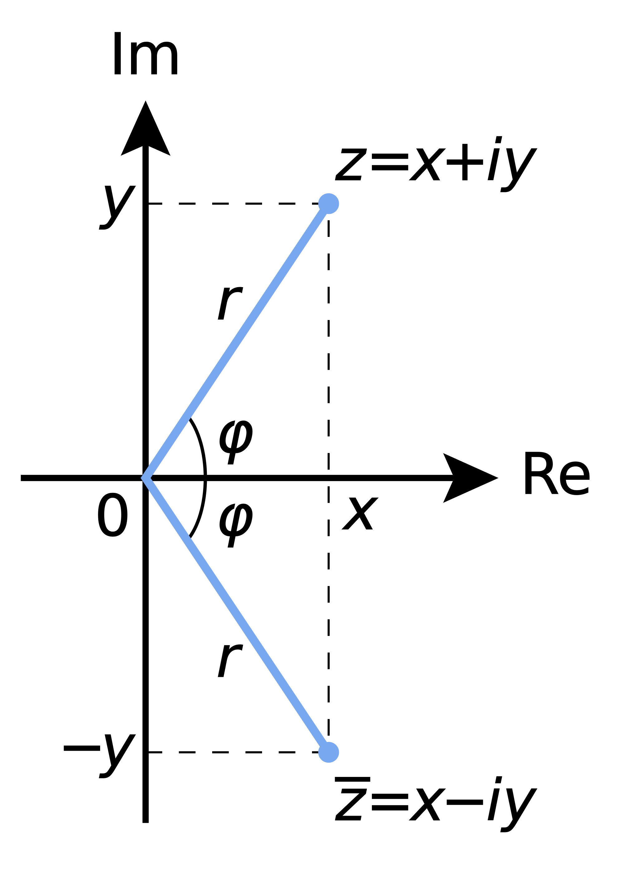
The first illustration just shows what a complex number really is: a two-dimensional number (z) with a real part (Re(z) = x) and an imaginary part (Im(z) = y). We can represent it in two ways: one uses the (x, y) coordinate system (z = x + iy), and the other is the so-called polar form: z = reⁱ^φ. The (real) number e in the latter equation is just Euler’s number, so that’s a mathematical constant (just like π). The little i is the imaginary unit, so that’s the thing we introduce to add a second (vertical) dimension to our analysis: i can be written as 0+i = (0, 1) indeed, and so it’s like a (second) basis vector in the two-dimensional (Cartesian or complex) plane.

I should not say much more about this, but I must list some essential properties and relationships:

The coordinate and polar form are related through Euler’s formula: z = x + iy = reⁱ^φ= r(cosφ + isinφ).
From this, and the fact that cos(-φ) = cosφ and sin(-φ) = –sinφ, it follows that the (complex) conjugate z* = x – iy of a complex number z = x + iy is equal to z* = re^–iφ. [I use z* as a symbol, instead of z-bar, because I can’t find a z-bar in the character set here.] This equality is illustrated above.
The length/modulus/absolute value of a complex number is written as |z| and is equal to |z| = (x² + y²)^1/2 = |reⁱ^φ| = r (so r is always a positive (real) number).
As you can see from the graph, a complex number z and its conjugate z* have the same absolute value: |z| = |x+iy| = |z*| = |x-iy|.
Therefore, we have the following: |z||z|=|z*||z*|=|z||z*|=|z|², and we can use this result to calculate the (multiplicative) inverse: z^-1 = 1/z = z*/|z|².
The absolute value of a product of complex numbers equals the product of the absolute values of those numbers: |z₁z₂| = |z₁||z₂|.
Last but not least, it is important to be aware of the geometric interpretation of the sum and the product of two complex numbers:
- The sum of two complex numbers amounts to adding vectors, so that’s the familiar parallelogram law for vector addition: (a+ib) + (c+id) = (a+b) + i(c+d).
- Multiplying two complex numbers amounts to adding the angles and multiplying their lengths – as evident from writing such product in its polar form: reⁱ^θseⁱ^Θ= rseⁱ⁽^θ+^Θ). The result is, quite obviously, another complex number. So it is not the usual scalar or vector product which you may or may not be familiar with.

[For the sake of completeness: (i) the scalar product (aka dot product) of two vectors (a•b) is equal to the product of is the product of the magnitudes of the two vectors and the cosine of the angle between them: a•b = |a||b|cosα; and (ii) the result of a vector product (or cross product) is a vector which is perpendicular to both, so it’s a vector that is not in the same plane as the vectors we are multiplying: a×b = |a||b| sinα n, with n the unit vector perpendicular to the plane containing a and b in the direction given by the so-called right-hand rule. Just be aware of the difference.]

The second illustration (see below) comes from that little book I mentioned above already: Feynman’s exquisite 1985 Alix G. Mautner Memorial Lectures on Quantum Electrodynamics, better known as QED: the Strange Theory of Light and Matter. It shows how these probability amplitudes, or ‘arrows’ as he calls them, really work, without even mentioning that they are ‘probability amplitudes’ or ‘complex numbers’. That being said, these ‘arrows’ are what they are: probability amplitudes.

To be precise, the illustration below shows the probability amplitude of a photon (so that’s a little packet of light) reflecting from the front surface (front reflection arrow) and the back (back reflection arrow) of a thin sheet of glass. If we write these vectors in polar form (reⁱ^φ), then it is obvious that they have the same length (r = 0.2) but their phase φ is different. That’s because the photon needs to travel a bit longer to reach the back of the glass: so the phase varies as a function of time and space, but the length doesn’t. Feynman visualizes that with the stopwatch: as the photon is emitted from a light source and travels through time and space, the stopwatch turns and, hence, the arrow will point in a different direction.

[To be even more precise, the amplitude for a photon traveling from point A to B is a (fairly simple) function (which I won’t write down here though) which depends on the so-called spacetime interval. This spacetime interval (written as I or s²) is equal to I = [(x₂-x₁)²+(y₂-y₁)²+(z₂-z₁)²] – (t₂-t₁)². So the first term in this expression is the square of the distance in space, and the second term is the difference in time, or the ‘time distance’. Of course, we need to measure time and distance in equivalent units: we do that either by measuring spatial distance in light-seconds (i.e. the distance traveled by light in one second) or by expressing time in units that are equal to the time it takes for light to travel one meter (in the latter case we ‘stretch’ time (by multiplying it with c, i.e. the speed of light) while in the former, we ‘stretch’ our distance units). Because of the minus sign between the two terms, the spacetime interval can be negative, zero, or positive, and we call these intervals time-like (I < 0), light-like (I = 0) or space-like (I > 0). Because nothing travels faster than light, two events separated by a space-like interval cannot have a cause-effect relationship. I won’t go into any more detail here but, at this point, you may want to read the article on the so-called light cone relating past and future events in Wikipedia, because that’s what we’re talking about here really.]

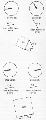
Feynman adds the two arrows, because a photon may be reflected either by the front surface or by the back surface and we can’t know which of the two possibilities was the case. So he adds the amplitudes here, not the probabilities. The probability of the photon bouncing off the front surface is the modulus of the amplitude squared, (i.e. |reⁱ^φ|²= r²), and so that’s 4% here (0.2·0.2). The probability for the back surface is the same: 4% also. However, the combined probability of a photon bouncing back from either the front or the back surface – we cannot know which path was followed – is not 8%, but some value between 0 and 16% (5% only in the top illustration, and 16% (i.e. the maximum) in the bottom illustration). This value depends on the thickness of the sheet of glass. That’s because it’s the thickness of the sheet that determines where the hand of our stopwatch stops. If the glass is just thick enough to make the stopwatch make one extra half turn as the photon travels through the glass from the front to the back, then we reach our maximum value of 16%, and so that’s what shown in the bottom half of the illustration above.

For the sake of completeness, I need to note that the full explanation is actually a bit more complex. Just a little bit. 🙂 Indeed, there is no such thing as ‘surface reflection’ really: a photon has an amplitude for scattering by each and every layer of electrons in the glass and so we have actually have many more arrows to add in order to arrive at a ‘final’ arrow. However, Feynman shows how all these arrows can be replaced by two so-called ‘radius arrows’: one for ‘front surface reflection’ and one for ‘back surface reflection’. The argument is relatively easy but I have no intention to fully copy Feynman here because the point here is only to illustrate how probabilities are calculated from probability amplitudes. So just remember: probabilities are real numbers between 0 and 1 (or between 0 and 100%), while amplitudes are complex numbers – or ‘arrows’ as Feynman calls them in this popular lectures series.

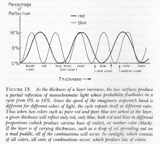
In order to give somewhat more credit to Feynman – and also to be somewhat more complete on how light really reflects from a sheet of glass (or a film of oil on water or a mud puddle), I copy one more illustration here – with the text – which speaks for itself: “The phenomenon of colors produced by the partial reflection of white light by two surfaces is called iridescence, and can be found in many places. Perhaps you have wondered how the brilliant colors of hummingbirds and peacocks are produced. Now you know.” The iridescence phenomenon is caused by really small variations in the thickness of the reflecting material indeed, and it is, perhaps, worth noting that Feynman is also known as the father of nanotechnology… 🙂

Light versus matter

So much for light – or electromagnetic waves in general. They consist of photons. Photons are discrete wave-packets of energy, and their energy (E) is related to the frequency of the light (f) through the Planck relation: E = hf. The factor h in this relation is the Planck constant, or the quantum of action in quantum mechanics as this tiny number (6.62606957×10⁻³⁴) is also being referred to. Photons have no mass and, hence, they travel at the speed of light indeed. But what about the other wave-like particles, like electrons?

For these, we have probability amplitudes (or, more generally, a wave function) as well, the characteristics of which are given by the de Broglie relations. These de Broglie relations also associate a frequency and a wavelength with the energy and/or the momentum of the ‘wave-particle’ that we are looking at: f = E/h and λ = h/p. In fact, one will usually find those two de Broglie relations in a slightly different but equivalent form: ω = E/ħ and k = p/ħ. The symbol ω stands for the angular frequency, so that’s the frequency expressed in radians. In other words, ω is the speed with which the hand of that stopwatch is going round and round and round. Similarly, k is the wave number, and so that’s the wavelength expressed in radians (or the spatial frequency one might say). We use k and ω in wave functions because the argument of these wave functions is the phase of the probability amplitude, and this phase is expressed in radians. For more details on how we go from distance and time units to radians, I refer to my previous post. [Indeed, I need to move on here otherwise this post will become a book of its own! Just check out the following: λ = 2π/k and f = ω/2π.]

How should we visualize a de Broglie wave for, let’s say, an electron? Well, I think the following illustration (which I took from Wikipedia) is not too bad.

Let’s first look at the graph on the top of the left-hand side of the illustration above. We have a complex wave function Ψ(x) here but only the real part of it is being graphed. Also note that we only look at how this function varies over space at some fixed point of time, and so we do not have a time variable here. That’s OK. Adding the complex part would be nice but it would make the graph even more ‘complex’ :-), and looking at one point in space only and analyzing the amplitude as a function of time only would yield similar graphs. If you want to see an illustration with both the real as well as the complex part of a wave function, have a look at my previous post.

We also have the probability – that’s the red graph – as a function of the probability amplitude: P = |Ψ(x)|² (so that’s just the modulus squared). What probability? Well, the probability that we can actually find the particle (let’s say an electron) at that location. Probability is obviously always positive (unlike the real (or imaginary) part of the probability amplitude, which oscillate around the x-axis). The probability is also reflected in the opacity of the little red ‘tennis ball’ representing our ‘wavicle’: the opacity varies as a function of the probability. So our electron is smeared out, so to say, over the space denoted as Δx.

Δx is the uncertainty about the position. The question mark next to the λ symbol (we’re still looking at the graph on the top left-hand side of the above illustration only: don’t look at the other three graphs now!) attributes this uncertainty to uncertainty about the wavelength. As mentioned in my previous post, wave packets, or wave trains, do not tend to have an exact wavelength indeed. And so, according to the de Broglie equation λ = h/p, if we cannot associate an exact value with λ, we will not be able to associate an exact value with p. Now that’s what’s shown on the right-hand side. In fact, because we’ve got a relatively good take on the position of this ‘particle’ (or wavicle we should say) here, we have a much wider interval for its momentum : Δp_x. [We’re only considering the horizontal component of the momentum vector p here, so that’s p_x.] $Φ(p) is referred to as the momentum wave function, and |Φ(p)| 2$ is the corresponding probability (or probability density as it’s usually referred to).

The two graphs at the bottom present the reverse situation: fairly precise momentum, but a lot of uncertainty about the wavicle’s position (I know I should stick to the term ‘particle’ – because that’s what physicists prefer – but I think ‘wavicle’ describes better what it’s supposed to be). So the illustration above is not only an illustration of the de Broglie wave function for a particle, but it also illustrates the Uncertainty Principle.

Now, I know I should move on to the thing I really want to write about in this post – i.e. bosons and fermions – but I feel I need to say a few things more about this famous ‘Uncertainty Principle’ – if only because I find it quite confusing. According to Feynman, one should not attach too much importance to it. Indeed, when introducing his simple arithmetic on probability amplitudes, Feynman writes the following about it: “The uncertainty principle needs to be seen in its historical context. When the revolutionary ideas of quantum physics were first coming out, people still tried to understand them in terms of old-fashioned ideas (such as, light goes in straight lines). But at a certain point, the old-fashioned ideas began to fail, so a warning was developed that said, in effect, ‘Your old-fashioned ideas are no damn good when…’ If you get rid of all the old-fashioned ideas and instead use the ideas that I’m explaining in these lectures – adding arrows for all the ways an event can happen – there is no need for the uncertainty principle!” So, according to Feynman, wave function math deals with all and everything and therefore we should, perhaps, indeed forget about this rather mysterious ‘principle’.

However, because it is mentioned so much (especially in the more popular writing), I did try to find some kind of easy derivation of its standard formulation: ΔxΔp ≥ ħ (ħ = h/2π, i.e. the quantum of angular momentum in quantum mechanics). To my surprise, it’s actually not easy to derive the uncertainty principle from other basic ‘principles’. As mentioned above, it follows from the de Broglie equation λ = h/p that momentum (p) and wavelength (λ) are related, but so how do we relate the uncertainty about the wavelength (Δλ) or the momentum (Δp) to the uncertainty about the position of the particle (Δx)? The illustration below, which analyzes a wave packet (aka a wave train), might provide some clue. Before you look at the illustration and start wondering what it’s all about, remember that a wave function with a definite (angular) frequency ω and wave number k (as described in my previous post), which we can write as Ψ = Ae^i(ωt-k•x), represents the amplitude of a particle with a known momentum p = ħ/k at some point x and t, and that we had a big problem with such wave, because the squared modulus of this function is a constant: |Ψ|² = |Ae^i(ωt-k•x)|²= A². So that means that the probability of finding this particle is the same at all points. So it’s everywhere and nowhere really (so it’s like the second wave function in the illustration above, but then with Δx infinitely long and the same wave shape all along the x-axis). Surely, we can’t have this, can we? Now we cannot – if only because of the fact that if we add up all of the probabilities, we would not get some finite number. So, in reality, particles are effectively confined to some region Δx or – if we limit our analysis to one dimension only (for the sake of simplicity) – Δx (remember that bold-type symbols represent vectors). So the probability amplitude of a particle is more likely to look like something that we refer to as a wave packet or a wave train. And so that’s what’s explained more in detail below.

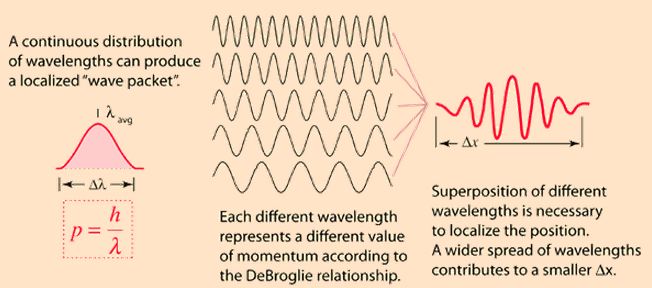
Now, I said that localized wave trains do not tend to have an exact wavelength. What do I mean with that? It doesn’t sound very precise, does it? In fact, we actually can easily sketch a graph of a wave packet with some fixed wavelength (or fixed frequency), so what am I saying here? I am saying that, in quantum physics, we are only looking at a very specific type of wave train: they are a composite of a (potentially infinite) number of waves whose wavelengths are distributed more or less continuously around some average, as shown in the illustration below, and so the addition of all of these waves – or their superposition as the process of adding waves is usually referred to – results in a combined ‘wavelength’ for the localized wave train that we cannot, indeed, equate with some exact number. I have not mastered the details of the mathematical process referred to as Fourier analysis (which refers to the decomposition of a combined wave into its sinusoidal components) as yet, and, hence, I am not in a position to quickly show you how Δx and Δλ are related exactly, but the point to note is that a wider spread of wavelengths results in a smaller Δx. Now, a wider spread of wavelengths corresponds to a wider spread in p too, and so there we have the Uncertainty Principle: the more we know about Δx, the less we know about Δx, and so that’s what the inequality ΔxΔp ≥ h/2π represents really.

[Those who like to check things out may wonder why a wider spread in wavelength implies a wider spread in momentum. Indeed, if we just replace λ and p with Δλ and Δp in the de Broglie equation λ = h/p, we get Δλ = h/Δp and so we have an inversely proportional relationship here, don’t we? No. We can’t just write that Δλ = Δ(h/p) but this Δ is not some mathematical operator than you can simply move inside of the brackets. What is Δλ? Is it a standard deviation? Is it the spread and, if so, what’s the spread? We could, for example, define it as the difference between some maximum value λ_maxand some minimum value λ_min, so as Δλ = λ_max– λ_min. These two values would then correspond with p_max=h/λ_min and p_min=h/λ_maxand so the corresponding spread in momentum would be equal to Δp = p_max– p_min = h/λ_min – h/λ_max= h(λ_max – λ_min)/(λ_maxλ_min). So a wider spread in wavelength does result in a wider spread in momentum, but the relationship is more subtle than you might think at first. In fact, in a more rigorous approach, we would indeed see the standard deviation (represented by the sigma symbol σ) from some average as a measure of the ‘uncertainty’. To be precise, the more precise formulation of the Uncertainty Principle is: σ_xσ_p≥ ħ/2, but don’t ask me where that 2 comes from!]

I really need to move on now, because this post is already way too lengthy and, hence, not very readable. So, back to that very first question: what’s that wave function math? Well, that’s obviously too complex a topic to be fully exhausted here. 🙂 I just wanted to present one aspect of it in this post: Bose-Einstein statistics. Huh? Yes.

When we say Bose-Einstein statistics, we should also say its opposite: Fermi-Dirac statistics. Bose-Einstein statistics were ‘discovered’ by the Indian scientist Satyanendra Nath Bose (the only thing Einstein did was to give Bose’s work on this wider recognition) and they apply to bosons (so they’re named after Bose only), while Fermi-Dirac statistics apply to fermions (‘Fermi-Diraqions’ doesn’t sound good either obviously). Any particle, or any wavicle I should say, is either a fermion or a boson. There’s a strict dichotomy: you can’t have characteristics of both. No split personalities. Not even for a split second.

The best-known examples of bosons are photons and the recently experimentally confirmed Higgs particle. But, in case you have heard of them, gluons (which mediate the so-called strong interactions between particles), and the W $+$ , W $-$ and Z particles (which mediate the so-called weak interactions) are bosons too. Protons, neutrons and electrons, on the other hand, are fermions.

More complex particles, such as atomic nuclei, are also either bosons or fermions. That depends on the number of protons and neutrons they consist of. But let’s not get ahead of ourselves. Here, I’ll just note that bosons – unlike fermions – can pile on top of one another without limit, all occupying the same ‘quantum state’. This explains superconductivity, superfluidity and Bose-Einstein condensation at low temperatures. Indeed, these phenomena usually involve (bosonic) helium. You can’t do it with fermions. Superfluid helium has very weird properties, including zero viscosity – so it flows without dissipating energy and it creeps up the wall of its container, seemingly defying gravity: just Google one of the videos on the Web! It’s amazing stuff! Bose statistics also explain why photons of the same frequency can form coherent and extremely powerful laser beams, with (almost) no limit as to how much energy can be focused in a beam.

Fermions, on the other hand, avoid one another. Electrons, for example, organize themselves in shells around a nucleus stack. They can never collapse into some kind of condensed cloud, as bosons can. If electrons would not be fermions, we would not have such variety of atoms with such great range of chemical properties. But, again, let’s not get ahead of ourselves. Back to the math.

Bose versus Fermi particles

When adding two probability amplitudes (instead of probabilities), we are adding complex numbers (or vectors or arrows or whatever you want to call them), and so we need to take their phase into account or – to put it simply – their direction. If their phase is the same, the length of the new vector will be equal to the sum of the lengths of the two original vectors. When their phase is not the same, then the new vector will be shorter than the sum of the lengths of the two amplitudes that we are adding. How much shorter? Well, that obviously depends on the angle between the two vectors, i.e. the difference in phase: if it’s 180 degrees (or π radians), then they will cancel each other out and we have zero amplitude! So that’s destructive or negative interference. If it’s less than 90 degrees, then we will have constructive or positive interference.

It’s because of this interference effect that we have to add probability amplitudes first, before we can calculate the probability of an event happening in one or the other (indistinguishable) way (let’s say A or B) – instead of just adding probabilities as we would do in the classical world. It’s not subtle. It makes a big difference: |Ψ_A + Ψ_B|²is the probability when we cannot distinguish the alternatives (so when we’re in the world of quantum mechanics and, hence, we have to add amplitudes), while |Ψ_A|²+ |Ψ_B|²is the probability when we can see what happens (i.e. we can see whether A or B was the case). Now, |Ψ_A + Ψ_B|²is definitely not the same as |Ψ_A|²+ |Ψ_B|²– not for real numbers, and surely not for complex numbers either. But let’s move on with the argument – literally: I mean the argument of the wave function at hand here.

That stopwatch business above makes it easier to introduce the thought experiment which Feynman also uses to introduce Bose versus Fermi statistics (Feynman Lectures (1965), Vol. III, Lecture 4). The experimental set-up is shown below. We have two particles, which are being referred to as particle a and particle b respectively (so we can distinguish the two), heading straight for each other and, hence, they are likely to collide and be scattered in some other direction. The experimental set-up is designed to measure where they are likely to end up, i.e. to measure probabilities. [There’s no certainty in the quantum-mechanical world, remember?] So, in this experiment, we have a detector (or counter) at location 1 and a detector/counter at location 2 and, after many many measurements, we have some value for the (combined) probability that particle a goes to detector 1 and particle b goes to counter 2. This amplitude is a complex number and you may expect it will depend on the angle θ as shown in the illustration below.

So this angle θ will obviously show up somehow in the argument of our wave function. Hence, the wave function, or probability amplitude, describing the amplitude of particle a ending up in counter 1 and particle b ending up in counter 2 will be some (complex) function Ψ₁= f(θ). Please note, once again, that θ is not some (complex) phase but some real number (expressed in radians) between 0 and 2π that characterizes the set-up of the experiment above. It is also worth repeating that f(θ) is not the amplitude of particle a hitting detector 1 only but the combined amplitude of particle a hitting counter 1 and particle b hitting counter 2! It makes a big difference and it’s essential in the interpretation of this argument! So, the combined probability of a going to 1 and of particle b going to 2, which we will write as P₁, is equal to |Ψ₁|²= |f(θ)|².

OK. That’s obvious enough. However, we might also find particle a in detector 2 and particle b in detector 1. Surely, the probability amplitude probability for this should be equal to f(θ+π)? It’s just a matter of switching counter 1 and 2 – i.e. we rotate their position over 180 degrees, or π (in radians) – and then we just insert the new angle of this experimental set-up (so that’s θ+π) into the very same wave function and there we are. Right?

Well… Maybe. The probability of a going to 2 and b going to 1, which we will write as P₂, will be equal to |f(θ+π)|²indeed. However, our probability amplitude, which I’ll write as Ψ₂, may not be equal to f(θ+π). It’s just a mathematical possibility. I am not saying anything definite here. Huh? Why not?

Well… Think about the thing we said about the phase and the possibility of a phase shift: f(θ+π) is just one of the many mathematical possibilities for a wave function yielding a probability P₂=|Ψ₂|²= |f(θ+π)|². But any function eⁱ^δf(θ+π) will yield the same probability. Indeed, |z₁z₂| = |z₁||z₂| and so |eⁱ^δ f(θ+π)|² = (|eⁱ^δ||f(θ+π)|)²= |eⁱ^δ|²|f(θ+π)|²= |f(θ+π)|²(the square of the modulus of a complex number on the unit circle is always one – because the length of vectors on the unit circle is equal to one). It’s a general thing: if Ψ is some wave function (i.e. it describes some complex amplitude in space and time, then eⁱ^δΨ is the same wave function but with a phase shift equal to δ. Huh? Yes. Think about it: we’re multiplying complex numbers here, so that’s adding angles and multiplying lengths. Now the length of eⁱ^δ is 1 (because it’s a complex number on the unit circle) but its phase is δ. So multiplying Ψ with eⁱ^δdoes not change the length of Ψ but it does shift its phase by an amount (in radians) equal to δ. That should be easy enough to understand.

You probably wonder what I am being so fussy, and what that δ could be, or why it would be there. After all, we do have a well-behaved wave function f(θ) here, depending on x, t and θ, and so the only thing we did was to change the angle θ (we added π radians to it). So why would we need to insert a phase shift here? Because that’s what δ really is: some random phase shift. Well… I don’t know. This phase factor is just a mathematical possibility as for now. So we just assume that, for some reason which we don’t understand right now, there might be some ‘arbitrary phase factor’ (that’s how Feynman calls δ) coming into play when we ‘exchange’ the ‘role’ of the particles. So maybe that δ is there, but maybe not. I admit it looks very ugly. In fact, if the story about Bose’s ‘discovery’ of this ‘mathematical possibility’ (in 1924) is correct, then it all started with an obvious ‘mistake’ in a quantum-mechanical calculation – but a ‘mistake’ that, miraculously, gave predictions that agreed with experimental results that could not be explained without introducing this ‘mistake’. So let the argument go full circle – literally – and take your time to appreciate the beauty of argumentation in physics.

Let’s swap detector 1 and detector 2 a second time, so we ‘exchange’ particle a and b once again. So then we need to apply this phase factor δ once again and, because of symmetry in physics, we obviously have to use the same phase factor δ – not some other value γ or something. We’re only rotating our detectors once again. That’s it. So all the rest stays the same. Of course, we also need to add π once more to the argument in our wave function f. In short, the amplitude for this is:

eⁱ^δ[eⁱ^δf(θ+π+π)] = (eⁱ^δ)²f(θ) = eⁱ²^δf(θ)

Indeed, the angle θ+2π is the same as θ. But so we have twice that phase shift now: 2δ. As ugly as that ‘thing’ above: eⁱ^δf(θ+π). However, if we square the amplitude, we get the same probability: P₁= |Ψ₁|²= |eⁱ²^δf(θ)| = |f(θ)|². So it must be right, right? Yes. But – Hey! Wait a minute! We are obviously back at where we started, aren’t we? We are looking at the combined probability – and amplitude – for particle a going to counter 1 and particle b going to counter 2, and the angle is θ! So it’s the same physical situation, and – What the heck! – reality doesn’t change just because we’re rotating these detectors a couple of times, does it? [In fact, we’re actually doing nothing but a thought experiment here!] Hence, not only the probability but also the amplitude must be the same. So (eⁱ^δ)²f(θ) must equal f(θ) and so… Well… If (eⁱ^δ)²f(θ) = f(θ), then (eⁱ^δ)² must be equal to 1. Now, what does that imply for the value of δ?

Well… While the square of the modulus of all vectors on the unit circle is always equal to 1, there are only two cases for which the square of the vector itself yields 1: (I) eⁱ^δ = eⁱ^π= e^–i^π = –1 (check it: (eⁱ^π)²= (–1)²= eⁱ²^π = eⁱ⁰ = +1), and (II) eⁱ^δ = eⁱ²^π= eⁱ⁰= e⁰= +1 (check it: eⁱ²^π)²= (+1)²= eⁱ⁴^π = eⁱ⁰ = +1). In other words, our phase factor δ is either δ = 0 (or 0 ± 2nπ) or, else, δ = π (or π ± 2nπ). So eⁱ^δ = ± 1 and Ψ₂ is either +f(θ+π) or, else, –f(θ+π). What does this mean? It means that, if we’re going to be adding the amplitudes, then the ‘exchanged case’ may contribute with the same sign or, else, with the opposite sign.

But, surely, there is no need to add amplitudes here, is there? Particle a can be distinguished from particle b and so the first case (particle a going into counter 1 and particle b going into counter 2) is not the same as the ‘exchanged case’ (particle a going into counter 2 and b going into counter 1). So we can clearly distinguish or verify which of the two possible paths are followed and, hence, we should be adding probabilities if we want to get the combined probability for both cases, not amplitudes. Now that is where the fun starts. Suppose that we have identical particles here – so not some beam of α-particles (i.e. helium nuclei) bombarding beryllium nuclei for instance but, let’s say, electrons on electrons, or photons on photons indeed – then we do have to add the amplitudes, not the probabilities, in order to calculate the combined probability of a particle going into counter 1 and the other particle going into counter 2, for the simple reason that we don’t know which is which and, hence, which is going where.

Let me immediately throw in an important qualifier: defining ‘identical particles’ is not as easy as it sounds. Our ‘wavicle’ of choice, for example, an electron, can have its spin ‘up’ or ‘down’ – and so that’s two different things. When an electron arrives in a counter, we can measure its spin (in practice or in theory: it doesn’t matter in quantum mechanics) and so we can distinguish it and, hence, an electron that’s ‘up’ is not identical to one that’s ‘down’. [I should resist the temptation but I’ll quickly make the remark: that’s the reason why we have two electrons in one atomic orbital: one is ‘up’ and the other one is ‘down’. Identical particles need to be in the same ‘quantum state’ (that’s the standard expression for it) to end up as ‘identical particles’ in, let’s say, a laser beam or so. As Feynman states it: in this (theoretical) experiment, we are talking polarized beams, with no mixture of different spin states.]

The wonderful thing in quantum mechanics is that mathematical possibility usually corresponds with reality. For example, electrons with positive charge, or anti-matter in general, is not only a theoretical possibility: they exist. Likewise, we effectively have particles which interfere with positive sign – these are called Bose particles – and particles which interfere with negative sign – Fermi particles.

So that’s reality. The factor eⁱ^δ = ± 1 is there, and it’s a strict dichotomy: photons, for example, always behave like Bose particles, and protons, neutrons and electrons always behave like Fermi particles. So they don’t change their mind and switch from one to the other category, not for a short while, and not for a long while (or forever) either. In fact, you may or may not be surprised to hear that there are experiments trying to find out if they do – just in case. 🙂 For example, just Google for Budker and English (2010) from the University of California at Berkeley. The experiments confirm the dichotomy: no split personalities here, not even for a nanosecond (10⁻⁹ s), or a picosecond (10⁻¹² s). [A picosecond is the time taken by light to travel 0.3 mm in a vacuum. In a nanosecond, light travels about one foot.]

In any case, does all of this really matter? What’s the difference, in practical terms that is? Between Bose or Fermi, I must assume we prefer the booze.

It’s quite fundamental, however. Hang in there for a while and you’ll see why.

Bose statistics

Suppose we have, once again, some particle a and b that (i) come from different directions (but, this time around, not necessarily in the experimental set-up as described above: the two particles may come from any direction really), (ii) are being scattered, at some point in space (but, this time around, not necessarily the same point in space), (iii) end up going in one and the same direction and – hopefully – (iv) arrive together at some other point in space. So they end up in the same state, which means they have the same direction and energy (or momentum) and also whatever other condition that’s relevant. Again, if the particles are not identical, we can catch both of them and identify which is which. Now, if it’s two different particles, then they won’t take exactly the same path. Let’s say they travel along two infinitesimally close paths referred to as path 1 and 2 and so we should have two infinitesimally small detectors: one at location 1 and the other at location 2. The illustration below (credit to Feynman once again!) is for n particles, but here we’ll limit ourselves to the calculations for just two.

Let’s denote the amplitude of a to follow path 1 (and end up in counter 1) as a₁, and the amplitude of b to follow path 2 (and end up in counter 2) as b₁. Then the amplitude for these two scatterings to occur at the same time is the product of these two amplitudes, and so the probability is equal to |a₁b₁|²= [|a₁||b₁|]²= |a₁|²|b₁|². Similarly, the combined amplitude of a following path 2 (and ending up in counter 2) and b following path 1 (etcetera) is |a₂|²|b₂|². But so we said that the directions 1 and 2 were infinitesimally close and, hence, the values for a₁and a₂, and for b₁and b₂, should also approach each other, so we can equate them with a and b respectively and, hence, the probability of some kind of combined detector picking up both particles as they hit the counter is equal to P = 2|a|²|b|² (just substitute and add). [Note: For those who would think that separate counters and ‘some kind of combined detector’ radically alter the set-up of this thought experiment (and, hence, that we cannot just do this kind of math), I refer to Feynman (Vol. III, Lecture 4, section 4): he shows how it works using differential calculus.]

Now, if the particles cannot be distinguished – so if we have ‘identical particles’ (like photons, or polarized electrons) – and if we assume they are Bose particles (so they interfere with a positive sign – i.e. like photons, but not like electrons), then we should no longer add the probabilities but the amplitudes, so we get a₁b₂+ a₂b₁= 2ab for the amplitude and – lo and behold! – a probability equal to P = 4|a|²|b|². So what? Well… We’ve got a factor 2 difference here: 4|a|²|b|²is two times 2|a|²|b|².

This is a strange result: it means we’re twice as likely to find two identical Bose particles scattered into the same state as you would assuming the particles were different. That’s weird, to say the least. In fact, it gets even weirder, because this experiment can easily be extended to a situation where we have n particles present (which is what the illustration suggests), and that makes it even more interesting (more ‘weird’ that is). I’ll refer to Feynman here for the (fairly easy but somewhat lengthy) calculus in case we have n particles, but the conclusion is rock-solid: if we have n bosons already present in some state, then the probability of getting one extra boson is n+1 times greater than it would be if there were none before.

So the presence of the other particles increases the probability of getting one more: bosons like to crowd. And there’s no limit to it: the more bosons you have in one space, the more likely it is another one will want to occupy the same space. It’s this rather weird phenomenon which explains equally weird things such as superconductivity and superfluidity, or why photons of the same frequency can form such powerful laser beams: they don’t mind being together – literally on the same spot – in huge numbers. In fact, they love it: a laser beam, superfluidity or superconductivity are actually quantum-mechanical phenomena that are visible at a macro-scale.

OK. I won’t go into any more detail here. Let me just conclude by showing how interference works for Fermi particles. Well… That doesn’t work or, let me be more precise, it leads to the so-called (Pauli) Exclusion Principle which, for electrons, states that “no two electrons can be found in exactly the same state (including spin).” Indeed, we get a₁b₂– a₂b₁= ab– ab = 0 (zero!) if we let the values of a₁and a₂, and b₁and b₂, come arbitrarily close to each other. So the amplitude becomes zero as the two directions (1 and 2) approach each other. That simply means that it is not possible at all for two electrons to have the same momentum, location or, in general, the same state of motion – unless they are spinning opposite to each other (in which case they are not ‘identical’ particles). So what? Well… Nothing much. It just explains all of the chemical properties of atoms. 🙂

In addition, the Pauli exclusion principle also explains the stability of matter on a larger scale: protons and neutrons are fermions as well, and so they just “don’t get close together with one big smear of electrons around them”, as Feynman puts it, adding: “Atoms must keep away from each other, and so the stability of matter on a large scale is really a consequence of the Fermi particle nature of the electrons, protons and neutrons.”

Well… There’s nothing much to add to that, I guess. 🙂

Post scriptum:

I wrote that “more complex particles, such as atomic nuclei, are also either bosons or fermions”, and that this depends on the number of protons and neutrons they consist of. In fact, bosons are, in general, particles with integer spin (0 or 1), while fermions have half-integer spin (1/2). Bosonic Helium-4 (He⁴) has zero spin. Photons (which mediate electromagnetic interactions), gluons (which mediate the so-called strong interactions between particles), and the W $+$ , W $-$ and Z particles (which mediate the so-called weak interactions) all have spin one (1). As mentioned above, Lithium-7 (Li⁷) has half-integer spin (3/2). The underlying reason for the difference in spin between He⁴ and Li⁷ is their composition indeed: He⁴ consists of two protons and two neutrons, while Li⁷consists of three protons and four neutrons.

However, we have to go beyond the protons and neutrons for some better explanation. We now know that protons and neutrons are not ‘fundamental’ any more: they consist of quarks, and quarks have a spin of 1/2. It is probably worth noting that Feynman did not know this when he wrote his Lectures in 1965, although he briefly sketches the findings of Murray Gell-Man and Georg Zweig, who published their findings in 1961 and 1964 only, so just a little bit before, and describes them as ‘very interesting’. I guess this is just another example of Feynman’s formidable intellect and intuition… In any case, protons and neutrons are so-called baryons: they consist of three quarks, as opposed to the short-lived (unstable) mesons, which consist of one quark and one anti-quark only (you may not have heard about mesons – they don’t live long – and so I won’t say anything about them). Now, an uneven number of quarks result in half-integer spin, and so that’s why protons and neutrons have half-integer spin. An even number of quarks result in integer spin, and so that’s why mesons have spin zero 0 or 1. Two protons and two neutrons together, so that’s He⁴, can condense into a bosonic state with spin zero, because four half-integer spins allows for an integer sum. Seven half-integer spins, however, cannot be combined into some integer spin, and so that’s why Li⁷ has half-integer spin (3/2). Electrons also have half-integer spin (1/2) too. So there you are.

Now, I must admit that this spin business is a topic of which I understand little – if anything at all. And so I won’t go beyond the stuff I paraphrased or quoted above. The ‘explanation’ surely doesn’t ‘explain’ this fundamental dichotomy between bosons and fermions. In that regard, Feynman’s 1965 conclusion still stands: “It appears to be one of the few places in physics where there is a rule which can be stated very simply, but for which no one has found a simple and easy explanation. The explanation is deep down in relativistic quantum mechanics. This probably means that we do not have a complete understanding of the fundamental principle involved. For the moment, you will just have to take it as one of the rules of the world.”

Some content on this page was disabled on June 20, 2020 as a result of a DMCA takedown notice from Michael A. Gottlieb, Rudolf Pfeiffer, and The California Institute of Technology. You can learn more about the DMCA here:

https://wordpress.com/support/copyright-and-the-dmca/
Some content on this page was disabled on June 20, 2020 as a result of a DMCA takedown notice from Michael A. Gottlieb, Rudolf Pfeiffer, and The California Institute of Technology. You can learn more about the DMCA here:

https://wordpress.com/support/copyright-and-the-dmca/

An easy piece: introducing quantum mechanics and the wave function

Pre-scriptum (dated 26 June 2020): A quick glance at this piece – so many years after I have written it – tells me it is basically OK. However, it is quite obvious that, in terms of interpreting the math, I have come a very long way. However, I would recommend you go through the piece so as to get the basic math, indeed, and then you may or may not be ready for the full development of my realist or classical interpretation of QM. My manuscript may also be a fun read for you.

Original post:

After all those boring pieces on math, it is about time I got back to physics. Indeed, what’s all that stuff on differential equations and complex numbers good for? This blog was supposed to be a journey into physics, wasn’t it? Yes. But wave functions – functions describing physical waves (in classical mechanics) or probability amplitudes (in quantum mechanics) – are the solution to some differential equation, and they will usually involve complex-number notation. However, I agree we have had enough of that now. Let’s see how it works. By the way, the title of this post – An Easy Piece – is an obvious reference to (some of) Feynman’s 1965 Lectures on Physics, some of which were re-packaged in 1994 (six years after his death that is) in ‘Six Easy Pieces’ indeed – but, IMHO, it makes more sense to read all of them as part of the whole series.

Let’s first look at one of the most used mathematical shapes: the sinusoidal wave. The illustration below shows the basic concepts: we have a wave here – some kind of cyclic thing – with a wavelength λ, an amplitude (or height) of (maximum) A₀, and a so-called phase shift equal to φ. The Wikipedia definition of a wave is the following: “a wave is a disturbance or oscillation that travels through space and matter, accompanied by a transfer of energy.” Indeed, a wave transports energy as it travels (oh – I forgot to mention the speed or velocity of a wave (v) as an important characteristic of a wave), and the energy it carries is directly proportional to the square of the amplitude of the wave: E ∝ A² (this is true not only for waves like water waves, but also for electromagnetic waves, like light).

Let’s now look at how these variables get into the argument – literally: into the argument of the wave function. Let’s start with that phase shift. The phase shift is usually defined referring to some other wave or reference point (in this case the origin of the x and y axis). Indeed, the amplitude – or ‘height’ if you want (think of a water wave, or the strength of the electric field) – of the wave above depends on (1) the time t (not shown above) and (2) the location (x), but so we will need to have this phase shift φ in the argument of the wave function because at x = 0 we do not have a zero height for the wave. So, as we can see, we can shift the x-axis left or right with this φ. OK. That’s simple enough. Let’s look at the other independent variables now: time and position.

The height (or amplitude) of the wave will obviously vary both in time as well as in space. On this graph, we fixed time (t = 0) – and so it does not appear as a variable on the graph – and show how the amplitude y = A varies in space (i.e. along the x-axis). We could also have looked at one location only (x = 0 or x₁or whatever other location) and shown how the amplitude varies over time at that location only. The graph would be very similar, except that we would have a ‘time distance’ between two crests (or between two troughs or between any other two points separated by a full cycle of the wave) instead of the wavelength λ (i.e. a distance in space). This ‘time distance’ is the time needed to complete one cycle and is referred to as the period of the wave (usually denoted by the symbol T or T₀– in line with the notation for the maximum amplitude A₀). In other words, we will also see time (t) as well as location (x) in the argument of this cosine or sine wave function. By the way, it is worth noting that it does not matter if we use a sine or cosine function because we can go from one to the other using the basic trigonometric identities cos θ = sin(π/2 – θ) and sin θ = cos(π/2 – θ). So all waves of the shape above are referred to as sinusoidal waves even if, in most cases, the convention is to actually use the cosine function to represent them.

So we will have x, t and φ in the argument of the wave function. Hence, we can write A = A(x, t, φ) = cos(x + t + φ) and there we are, right? Well… No. We’re adding very different units here: time is measured in seconds, distance in meter, and the phase shift is measured in radians (i.e. the unit of choice for angles). So we can’t just add them up. The argument of a trigonometric function (like this cosine function) is an angle and, hence, we need to get everything in radians – because that’s the unit we use to measure angles. So how do we do that? Let’s do it step by step.

First, it is worth noting that waves are usually caused by something. For example, electromagnetic waves are caused by an oscillating point charge somewhere, and radiate out from there. Physical waves – like water waves, or an oscillating string – usually also have some origin. In fact, we can look at a wave as a way of transmitting energy originating elsewhere. In the case at hand here – i.e. the nice regular sinusoidal wave illustrated above – it is obvious that the amplitude at some time t = t₁at some point x = x₁ will be the same as the amplitude of that wave at point x = 0 some time ago. How much time ago? Well… The time (t₀) that was needed for that wave to travel from point x = 0 to point x = x₁is easy to calculate: indeed, if the wave originated at t = 0 and x = 0, then x₁(i.e. the distance traveled by the wave) will be equal to its velocity (v) multiplied by t₁, so we have x₁= v.t₁(note that we assume the wave velocity is constant – which is a very reasonable assumption). In other words, inserting x₁and t₁ in the argument of our cosine function should yield the same value as inserting zero for x and t. Distance and time can be substituted so to say, and that’s we will have something like x – vt or vt – x in the argument in that cosine function: we measure both time and distance in units of distance so to say. [Note that x – vt and –(x-vt) = vt – x are equivalent because cos θ = cos (-θ)]

Does this sound fishy? It shouldn’t. Think about it. In the (electric) field equation for electromagnetic radiation (that’s one of the examples of a wave which I mentioned above), you’ll find the so-called retarded acceleration a(t – x/c) in the argument: that’s the acceleration (a)of the charge causing the electric field at point x to change not at time t but at time t – x/c. So that’s the retarded acceleration indeed: x/c is the time it took for the wave to travel from its origin (the oscillating point charge) to x and so we subtract that from t. [When talking electromagnetic radiation (e.g. light), the wave velocity v is obviously equal to c, i.e. the speed of light, or of electromagnetic radiation in general.] Of course, you will now object that t – x/c is not the same as vt – x, and you are right: we need time units in the argument of that acceleration function, not distance. We can get to distance units if we would multiply the time with the wave velocity v but that’s complicated business because the velocity of that moving point charge is not a constant.

[…] I am not sure if I made myself clear here. If not, so be it. The thing to remember is that we need an input expressed in radians for our cosine function, not time, nor distance. Indeed, the argument in a sine or cosine function is an angle, not some distance. We will call that angle the phase of the wave, and it is usually denoted by the symbol θ – which we also used above. But so far we have been talking about amplitude as a function of distance, and we expressed time in distance units too – by multiplying it with v. How can we go from some distance to some angle? It is simple: we’ll multiply x – vt with 2π/λ.

Huh? Yes. Think about it. The wavelength will be expressed in units of distance – typically 1 m in the SI International System of Units but it could also be angstrom (10^–10 m = 0.1 nm) or nano-meter (10^–9 m = 10 Å). A wavelength of two meter (2 m) means that the wave only completes half a cycle per meter of travel. So we need to translate that into radians, which – once again – is the measure used to… well… measure angles, or the phase of the wave as we call it here. So what’s the ‘unit’ here? Well… Remember that we can add or subtract 2π (and any multiple of 2π, i.e. ± 2nπ with n = ±1, ±2, ±3,…) to the argument of all trigonometric functions and we’ll get the same value as for the original argument. In other words, a cycle characterized by a wavelength λ corresponds to the angle θ going around the origin and describing one full circle, i.e. 2π radians. Hence, it is easy: we can go from distance to radians by multiplying our ‘distance argument’ x – vt with 2π/λ. If you’re not convinced, just work it out for the example I gave: if the wavelength is 2 m, then 2π/λ equals 2π/2 = π. So traveling 6 meters along the wave – i.e. we’re letting x go from 0 to 6 m while fixing our time variable – corresponds to our phase θ going from 0 to 6π: both the ‘distance argument’ as well as the change in phase cover three cycles (three times two meter for the distance, and three times 2π for the change in phase) and so we’re fine. [Another way to think about it is to remember that the circumference of the unit circle is also equal to 2π (2π·r = 2π·1 in this case), so the ratio of 2π to λ measures how many times the circumference contains the wavelength.]

In short, if we put time and distance in the (2π/λ)(x-vt) formula, we’ll get everything in radians and that’s what we need for the argument for our cosine function. So our sinusoidal wave above can be represented by the following cosine function:

A = A(x, t) = A₀cos[(2π/λ)(x-vt)]

We could also write A = A₀cosθ with θ = (2π/λ)(x-vt). […] Both representations look rather ugly, don’t they? They do. And it’s not only ugly: it’s not the standard representation of a sinusoidal wave either. In order to make it look ‘nice’, we have to introduce some more concepts here, notably the angular frequency and the wave number. So let’s do that.

The angular frequency is just like the… well… the frequency you’re used to, i.e. the ‘non-angular’ frequency f, as measured in cycles per second (i.e. in Hertz). However, instead of measuring change in cycles per second, the angular frequency (usually denoted by the symbol ω) will measure the rate of change of the phase with time, so we can write or define ω as ω = ∂θ/∂t. In this case, we can easily see that ω = –2πv/λ. [Note that we’ll take the absolute value of that derivative because we want to work with positive numbers for such properties of functions.] Does that look complicated? In doubt, just remember that ω is measured in radians per second and then you can probably better imagine what it is really. Another way to understand ω somewhat better is to remember that the product of ω and the period T is equal to 2π, so that’s a full cycle. Indeed, the time needed to complete one cycle multiplied with the phase change per second (i.e. per unit time) is equivalent to going round the full circle: 2π = ω.T. Because f = 1/T, we can also relate ω to f and write ω = 2π.f = 2π/T.

Likewise, we can measure the rate of change of the phase with distance, and that gives us the wave number k = ∂θ/∂x, which is like the spatial frequency of the wave. So it is just like the wavelength but then measured in radians per unit distance. From the function above, it is easy to see that k = 2π/λ. The interpretation of this equality is similar to the ω.T = 2π equality. Indeed, we have a similar equation for k: 2π = k.λ, so the wavelength (λ) is for k what the period (T) is for ω. If you’re still uncomfortable with it, just play a bit with some numerical examples and you’ll be fine.

To make a long story short, this, then, allows us to re-write the sinusoidal wave equation above in its final form (and let me include the phase shift φ again in order to be as complete as possible at this stage):

A(x, t) = A₀cos(kx – ωt + φ)

You will agree that this looks much ‘nicer’ – and also more in line with what you’ll find in textbooks or on Wikipedia. 🙂 I should note, however, that we’re not adding any new parameters here. The wave number k and the angular frequency ω are not independent: this is still the same wave (A = A₀cos[(2π/λ)(x-vt)]), and so we are not introducing anything more than the frequency and – equally important – the speed with which the wave travels, which is usually referred to as the phase velocity. In fact, it is quite obvious from the ω.T = 2π and the k = 2π/λ identities that kλ = ω.T and, hence, taking into account that λ is obviously equal to λ = v.T (the wavelength is – by definition – the distance traveled by the wave in one period), we find that the phase (or wave) velocity v is equal to the ratio of ω and k, so we have that v = ω/k. So x, t, ω and k could be re-scaled or so but their ratio cannot change: the velocity of the wave is what it is. In short, I am introducing two new concepts and symbols (ω and k) but there are no new degrees of freedom in the system so to speak.

[At this point, I should probably say something about the difference between the phase velocity and the so-called group velocity of a wave. Let me do that in as brief a way as I can manage. Most real-life waves travel as a wave packet, aka a wave train. So that’s like a burst, or an “envelope” (I am shamelessly quoting Wikipedia here…), of “localized wave action that travels as a unit.” Such wave packet has no single wave number or wavelength: it actually consists of a (large) set of waves with phases and amplitudes such that they interfere constructively only over a small region of space, and destructively elsewhere. The famous Fourier analysis (or infamous if you have problems understanding what it is really) decomposes this wave train in simpler pieces. While these ‘simpler’ pieces – which, together, add up to form the wave train – are all ‘nice’ sinusoidal waves (that’s why I call them ‘simple’), the wave packet as such is not. In any case (I can’t be too long on this), the speed with which this wave train itself is traveling through space is referred to as the group velocity. The phase velocity and the group velocity are usually very different: for example, a wave packet may be traveling forward (i.e. its group velocity is positive) but the phase velocity may be negative, i.e. traveling backward. However, I will stop here and refer to the Wikipedia article on group and phase velocity: it has wonderful illustrations which are much and much better than anything I could write here. Just one last point that I’ll use later: regardless of the shape of the wave (sinusoidal, sawtooth or whatever), we have a very obvious relationship relating wavelength and frequency to the (phase) velocity: v = λ.f, or f = v/λ. For example, the frequency of a wave traveling 3 meter per second and wavelength of 1 meter will obviously have a frequency of three cycles per second (i.e. 3 Hz). Let’s go back to the main story line now.]

With the rather lengthy ‘introduction’ to waves above, we are now ready for the thing I really wanted to present here. I will go much faster now that we have covered the basics. Let’s go.

From my previous posts on complex numbers (or from what you know on complex numbers already), you will understand that working with cosine functions is much easier when writing them as the real part of a complex number A₀eⁱ^θ= A₀eⁱ^{(kx –}^{ωt + φ)}. Indeed, A₀eⁱ^θ = A₀(cosθ + isinθ) and so the cosine function above is nothing else but the real part of the complex number A₀eⁱ^θ. Working with complex numbers makes adding waves and calculating interference effects and whatever we want to do with these wave functions much easier: we just replace the cosine functions by complex numbers in all of the formulae, solve them (algebra with complex numbers is very straightforward), and then we look at the real part of the solution to see what is happening really. We don’t care about the imaginary part, because that has no relationship to the actual physical quantities – for physical and electromagnetic waves that is, or for any other problem in classical wave mechanics. Done. So, in classical mechanics, the use of complex numbers is just a mathematical tool.

Now, that is not the case for the wave functions in quantum mechanics: the imaginary part of a wave equation – yes, let me write one down here – such as Ψ = Ψ(x, t) = (1/x)eⁱ^{(kx – ωt)}is very much part and parcel of the so-called probability amplitude that describes the state of the system here. In fact, this Ψ function is an example taken from one of Feynman’s first Lectures on Quantum Mechanics (i.e. Volume III of his Lectures) and, in this case, Ψ(x, t) = (1/x)eⁱ^{(kx – ωt)}represents the probability amplitude of a tiny particle (e.g. an electron) moving freely through space – i.e. without any external forces acting upon it – to go from 0 to x and actually be at point x at time t. [Note how it varies inversely with the distance because of the 1/x factor, so that makes sense.] In fact, when I started writing this post, my objective was to present this example – because it illustrates the concept of the wave function in quantum mechanics in a fairly easy and relatively understandable way. So let’s have a go at it.

First, it is necessary to understand the difference between probabilities and probability amplitudes. We all know what a probability is: it is a real number between o and 1 expressing the chance of something happening. It is usually denoted by the symbol P. An example is the probability that monochromatic light (i.e. one or more photons with the same frequency) is reflected from a sheet of glass. [To be precise, this probability is anything between 0 and 16% (i.e. P = 0 to 0.16). In fact, this example comes from another fine publication of Richard Feynman – QED (1985) – in which he explains how we can calculate the exact probability, which depends on the thickness of the sheet.]

A probability amplitude is something different. A probability amplitude is a complex number (3 + 2i, or 2.6eⁱ^1.34, for example) and – unlike its equivalent in classical mechanics – both the real and imaginary part matter. That being said, probabilities and probability amplitudes are obviously related: to be precise, one calculates the probability of an event actually happening by taking the square of the modulus (or the absolute value) of the probability amplitude associated with that event. Huh? Yes. Just let it sink in. So, if we denote the probably amplitude by Φ, then we have the following relationship:

P =|Φ|²

P = probability

Φ = probability amplitude

In addition, where we would add and multiply probabilities in the classical world (for example, to calculate the probability of an event which can happen in two different ways – alternative 1 and alternative 2 let’s say – we would just add the individual probabilities to arrive at the probably of the event happening in one or the other way, so P = P₁+ P₂), in the quantum-mechanical world we should add and multiply probability amplitudes, and then take the square of the modulus of that combined amplitude to calculate the combined probability. So, formally, the probability of a particle to reach a given state by two possible routes (route 1 or route 2 let’s say) is to be calculated as follows:

Φ = Φ₁+ Φ₂

and P =|Φ|²=|Φ₁+ Φ₂|²

Also, when we have only one route, but that one route consists of two successive stages (for example: to go from A to C, the particle would have first have to go from A to B, and then from B to C, with different probabilities of stage AB and stage BC actually happening), we will not multiply the probabilities (as we would do in the classical world) but the probability amplitudes. So we have:

Φ = Φ_ABΦ_BC

and P =|Φ|²=|Φ_ABΦ_BC|²

In short, it’s the probability amplitudes (and, as mentioned, these are complex numbers, not real numbers) that are to be added and multiplied etcetera and, hence, the probability amplitudes act as the equivalent, so to say, in quantum mechanics, of the conventional probabilities in classical mechanics. The difference is not subtle. Not at all. I won’t dwell too much on this. Just re-read any account of the double-slit experiment with electrons which you may have read and you’ll remember how fundamental this is. [By the way, I was surprised to learn that the double-slit experiment with electrons has apparently only been done in 2012 in exactly the way as Feynman described it. So when Feynman described it in his 1965 Lectures, it was still very much a ‘thought experiment’ only – even a 1961 experiment (not mentioned by Feynman) had clearly established the reality of electron interference.]

OK. Let’s move on. So we have this complex wave function in quantum mechanics and, as Feynman writes, “It is not like a real wave in space; one cannot picture any kind of reality to this wave as one does for a sound wave.” That being said, one can, however, get pretty close to ‘imagining’ what it actually is IMHO. Let’s go by the example which Feynman gives himself – on the very same page where he writes the above actually. The amplitude for a free particle (i.e. with no forces acting on it) with momentum p = mv to go from location r₁to location r₂is equal to

Φ₁₂= (1/r₁₂)eⁱ^p.r₁₂/ħwith r₁₂ = r₂– r₁

I agree this looks somewhat ugly again, but so what does it say? First, be aware of the difference between bold and normal type: I am writing p and v in bold type above because they are vectors: they have a magnitude (which I will denote by p and v respectively) as well as a direction in space. Likewise, r₁₂ is a vector going from r₁to r₂ (and r₁and r₂ themselves are space vectors themselves obviously) and so r₁₂(non-bold) is the magnitude of that vector. Keeping that in mind, we know that the dot product p.r₁₂ is equal to the product of the magnitudes of those vectors multiplied by cosα, with α the angle between those two vectors. Hence, p.r₁₂ .= p.r₁₂.cosα. Now, if p and r₁₂ have the same direction, the angle α will be zero and so cosα will be equal to one and so we just have p.r₁₂ = p.r₁₂or, if we’re considering a particle going from 0 to some position x, p.r₁₂ = p.r₁₂= px.

Now we also have Planck’s constant there, in its reduced form ħ = h/2π. As you can imagine, this 2π has something to do with the fact that we need radians in the argument. It’s the same as what we did with x in the argument of that cosine function above: if we have to express stuff in radians, then we have to absorb a factor of 2π in that constant. However, here I need to make an additional digression. Planck’s constant is obviously not just any constant: it is the so-called quantum of action. Indeed, it appears in what may well the most fundamental relations in physics.

The first of these fundamental relations is the so-called Planck relation: E = hf. The Planck relation expresses the wave-particle duality of light (or electromagnetic waves in general): light comes in discrete quanta of energy (photons), and the energy of these ‘wave particles’ is directly proportional to the frequency of the wave, and the factor of proportionality is Planck’s constant.

The second fundamental relation, or relations – in plural – I should say, are the de Broglie relations. Indeed, Louis-Victor-Pierre-Raymond, 7th duc de Broglie, turned the above on its head: if the fundamental nature of light is (also) particle-like, then the fundamental nature of particles must (also) be wave-like. So he boldly associated a frequency f and a wavelength λ with all particles, such as electrons for example – but larger-scale objects, such as billiard balls, or planets, also have a de Broglie wavelength and frequency! The de Broglie relation determining the de Broglie frequency is – quite simply – the re-arranged Planck relation: f = E/h. So this relation relates the de Broglie frequency with energy. However, in the above wave function, we’ve got momentum, not energy. Well… Energy and momentum are obviously related, and so we have a second de Broglie relation relating momentum with wavelength: λ = h/p.

We’re almost there: just hang in there. 🙂 When we presented the sinusoidal wave equation, we introduced the angular frequency (ω) and the wave number (k), instead of working with f and λ. That’s because we want an argument expressed in radians. Here it’s the same. The two de Broglie equations have a equivalent using angular frequency and wave number: ω = E/ħ and k = p/ħ. So we’ll just use the second one (i.e. the relation with the momentum in it) to associate a wave number with the particle (k = p/ħ).

Phew! So, finally, we get that formula which we introduced a while ago already: Ψ(x) = (1/x)eⁱ^kx, or, including time as a variable as well (we made abstraction of time so far):

Ψ(x, t) = (1/x)eⁱ^{(kx – ωt)}

The formula above obviously makes sense. For example, the 1/x factor makes the probability amplitude decrease as we get farther away from where the particle started: in fact, this 1/x or 1/r variation is what we see with electromagnetic waves as well: the amplitude of the electric field vector E varies as 1/r and, because we’re talking some real wave here and, hence, its energy is proportional to the square of the field, the energy that the source can deliver varies inversely as the square of the distance. [Another way of saying the same is that the energy we can take out of a wave within a given conical angle is the same, no matter how far away we are: the energy flux is never lost – it just spreads over a greater and greater effective area. But let’s go back to the main story.]

We’ve got the math – I hope. But what does this equation mean really? What’s that de Broglie wavelength or frequency in reality? What wave are we talking about? Well… What’s reality? As mentioned above, the famous de Broglie relations associate a wavelength λ and a frequency f to a particle with momentum p and energy E, but it’s important to mention that the associated de Broglie wave function yields probability amplitudes. So it is, indeed, not a ‘real wave in space’ as Feynman would put it. It is a quantum-mechanical wave equation.

Huh? […] It’s obviously about time I add some illustrations here, and so that’s what I’ll do. Look at the two cases below. The case on top is pretty close to the situation I described above: it’s a de Broglie wave – so that’s a complex wave – traveling through space (in one dimension only here). The real part of the complex amplitude is in blue, and the green is the imaginary part. So the probability of finding that particle at some position x is the modulus squared of this complex amplitude. Now, this particular wave function ignores the 1/x variation and, hence, the squared modulus of Aeⁱ^{(kx – ωt)}is equal to a constant. To be precise, it’s equal to A² (check it: the squared modulus of a complex number z equals the product of z and its complex conjugate, and so we get A²as a result indeed). So what does this mean? It means that the probability of finding that particle (an electron, for example) is the same at all points! In other words, we don’t know where it is! In the illustration below (top part), that’s shown as the (yellow) color opacity: the probability is spread out, just like the wave itself, so there is no definite position of the particle indeed.

[Note that the formula in the illustration above (which I took from Wikipedia once again) uses p instead of k as the factor in front of x. While it does not make a big difference from a mathematical point of view (ħ is just a factor of proportionality: k = p/ħ), it does make a big difference from a conceptual point of view and, hence, I am puzzled as to why the author of this article did this. Also, there is some variation in the opacity of the yellow (i.e. the color of our tennis (or ping pong) ball representing our ‘wavicle’) which shouldn’t be there because the probability associated with this particular wave function is a constant indeed: so there is no variation in the probability (when squaring the absolute value of a complex number, the phase factor does not come into play). Also note that, because all probabilities have to add up to 100% (or to 1), a wave function like this is quite problematic. However, don’t worry about it just now: just try to go with the flow.]

By now, I must assume you shook your head in disbelief a couple of time already. Surely, this particle (let’s stick to the example of an electron) must be somewhere, yes? Of course.

The problem is that we gave an exact value to its momentum and its energy and, as a result, through the de Broglie relations, we also associated an exact frequency and wavelength to the de Broglie wave associated with this electron. Hence, Heisenberg’s Uncertainty Principle comes into play: if we have exact knowledge on momentum, then we cannot know anything about its location, and so that’s why we get this wave function covering the whole space, instead of just some region only. Sort of. Here we are, of course, talking about that deep mystery about which I cannot say much – if only because so many eminent physicists have already exhausted the topic. I’ll just state Feynman once more: “Things on a very small scale behave like nothing that you have any direct experience with. […] It is very difficult to get used to, and it appears peculiar and mysterious to everyone – both to the novice and to the experienced scientist. Even the experts do not understand it the way they would like to, and it is perfectly reasonable that they should not because all of direct, human experience and of human intuition applies to large objects. We know how large objects will act, but things on a small scale just do not act that way. So we have to learn about them in a sort of abstract or imaginative fashion and not by connection with our direct experience.” And, after describing the double-slit experiment, he highlights the key conclusion: “In quantum mechanics, it is impossible to predict exactly what will happen. We can only predict the odds [i.e. probabilities]. Physics has given up on the problem of trying to predict exactly what will happen. Yes! Physics has given up. We do not know how to predict what will happen in a given circumstance. It is impossible: the only thing that can be predicted is the probability of different events. It must be recognized that this is a retrenchment in our ideal of understanding nature. It may be a backward step, but no one has seen a way to avoid it.”

[…] That’s enough on this I guess, but let me – as a way to conclude this little digression – just quickly state the Uncertainty Principle in a more or less accurate version here, rather than all of the ‘descriptions’ which you may have seen of it: the Uncertainty Principle refers to any of a variety of mathematical inequalities asserting a fundamental limit (fundamental means it’s got nothing to do with observer or measurement effects, or with the limitations of our experimental technologies) to the precision with which certain pairs of physical properties of a particle (these pairs are known as complementary variables) such as, for example, position (x) and momentum (p), can be known simultaneously. More in particular, for position and momentum, we have that σ_xσ_p ≥ ħ/2 (and, in this formulation, σ is, obviously the standard symbol for the standard deviation of our point estimate for x and p respectively).

OK. Back to the illustration above. A particle that is to be found in some specific region – rather than just ‘somewhere’ in space – will have a probability amplitude resembling the wave equation in the bottom half: it’s a wave train, or a wave packet, and we can decompose it, using the Fourier analysis, in a number of sinusoidal waves, but so we do not have a unique wavelength for the wave train as a whole, and that means – as per the de Broglie equations – that there’s some uncertainty about its momentum (or its energy).

I will let this sink in for now. In my next post, I will write some more about these wave equations. They are usually a solution to some differential equation – and that’s where my next post will connect with my previous ones (on differential equations). Just to say goodbye – as for now that is – I will just copy another beautiful illustration from Wikipedia. See below: it represents the (likely) space in which a single electron on the 5d atomic orbital of a hydrogen atom would be found. The solid body shows the places where the electron’s probability density (so that’s the squared modulus of the probability amplitude) is above a certain value – so it’s basically the area where the likelihood of finding the electron is higher than elsewhere. The hue on the colored surface shows the complex phase of the wave function.

It is a wonderful image, isn’t it? At the very least, it increased my understanding of the mystery surround quantum mechanics somewhat. I hope it helps you too. 🙂

Post scriptum 1: On the need to normalize a wave function

In this post, I wrote something about the need for probabilities to add up to 1. In mathematical terms, this condition will resemble something like

In this integral, we’ve got – once again – the squared modulus of the wave function, and so that’s the probability of find the particle somewhere. The integral just states that all of the probabilities added all over space (Rⁿ) should add up to some finite number (a²). Hey! But that’s not equal to 1 you’ll say. Well… That’s a minor problem only: we can create a normalized wave function ψ out of ψ₀ by simply dividing $ψ by a so we have ψ = ψ 0 / a, and then all is ‘normal’ indeed. 🙂$

Post scriptum 2: On using colors to represent complex numbers

When inserting that beautiful 3D graph of that 5d atomic orbital (again acknowledging its source: Wikipedia), I wrote that “the hue on the colored surface shows the complex phase of the wave function.” Because this kind of visual representation of complex numbers will pop up in other posts as well (and you’ve surely encountered it a couple of times already), it’s probably useful to be explicit on what it represents exactly. Well… I’ll just copy the Wikipedia explanation, which is clear enough: “Given a complex number z = re^iθ, the phase (also known as argument) θ can be represented by a hue, and the modulus r =|z| is represented by either intensity or variations in intensity. The arrangement of hues is arbitrary, but often it follows the color wheel. Sometimes the phase is represented by a specific gradient rather than hue.” So here you go…

Post scriptum 3: On the de Broglie relations

The de Broglie relations are a wonderful pair. They’re obviously equivalent: energy and momentum are related, and wavelength and frequency are obviously related too through the general formula relating frequency, wavelength and wave velocity: fλ = v (the product of the frequency and the wavelength must yield the wave velocity indeed). However, when it comes to the relation between energy and momentum, there is a little catch. What kind of energy are we talking about? We were describing a free particle (e.g. an electron) traveling through space, but with no (other) charges acting on it – in other words: no potential acting upon it), and so we might be tempted to conclude that we’re talking about the kinetic energy (K.E.) here. So, at relatively low speeds (v), we could be tempted to use the equations p = mv and K.E. = p²/2m = mv²/2 (the one electron in a hydrogen atom travels at less than 1% of the speed of light, and so that’s a non-relativistic speed indeed) and try to go from one equation to the other with these simple formulas. Well… Let’s try it.

f = E/h according to de Broglie and, hence, substituting E with p²/2m and f with v/λ, we get v/λ = m²v²/2mh. Some simplification and re-arrangement should then yield the second de Broglie relation: λ = 2h/mv = 2h/p. So there we are. Well… No. The second de Broglie relation is just λ = h/p: there is no factor 2 in it. So what’s wrong? The problem is the energy equation: de Broglie does not use the K.E. formula. [By the way, you should note that the K.E. = mv²/2 equation is only an approximation for low speeds – low compared to c that is.] He takes Einstein’s famous E = mc²equation (which I am tempted to explain now but I won’t) and just substitutes c, the speed of light, with v, the velocity of the slow-moving particle. This is a very fine but also very deep point which, frankly, I do not yet fully understand. Indeed, Einstein’s E = mc²is obviously something much ‘deeper’ than the formula for kinetic energy. The latter has to do with forces acting on masses and, hence, obeys Newton’s laws – so it’s rather familiar stuff. As for Einstein’s formula, well… That’s a result from relativity theory and, as such, something that is much more difficult to explain. While the difference between the two energy formulas is just a factor of 1/2 (which is usually not a big problem when you’re just fiddling with formulas like this), it makes a big conceptual difference.

Hmm… Perhaps we should do some examples. So these de Broglie equations associate a wave with frequency f and wavelength λ with particles with energy E, momentum p and mass m traveling through space with velocity v: E = hf and p = h/λ. [And, if we would want to use some sine or cosine function as an example of such wave function – which is likely – then we need an argument expressed in radians rather than in units of time or distance. In other words, we will need to convert frequency and wavelength to angular frequency and wave number respectively by using the 2π = ωT = ω/f and 2π = kλ relations, with the wavelength (λ), the period (T) and the velocity (v) of the wave being related through the simple equations f = 1/T and λ = vT. So then we can write the de Broglie relations as: E = ħω and p = ħk, with ħ = h/2π.]

In these equations, the Planck constant (be it h or ħ) appears as a simple factor of proportionality (we will worry about what h actually is in physics in later posts) – but a very tiny one: approximately 6.626×10^–34 J·s (Joule is the standard SI unit to measure energy, or work: 1 J = 1 kg·m²/s²), or 4.136×10^–15 eV·s when using a more appropriate (i.e. larger) measure of energy for atomic physics: still, 10^–15 is only 0.000 000 000 000 001. So how does it work? First note, once again, that we are supposed to use the equivalent for slow-moving particles of Einstein’s famous E = mc²equation as a measure of the energy of a particle: E = mv². We know velocity adds mass to a particle – with mass being a measure for inertia. In fact, the mass of so-called massless particles, like photons, is nothing but their energy (divided by c²). In other words, they do not have a rest mass, but they do have a relativistic mass m = E/c², with E = hf (and with f the frequency of the light wave here). Particles, such as electrons, or protons, do have a rest mass, but then they don’t travel at the speed of light. So how does that work out in that E = mv²formula which – let me emphasize this point once again – is not the standard formula (for kinetic energy) that we’re used to (i.e. E = mv²/2)? Let’s do the exercise.

For photons, we can re-write E = hf as E = hc/λ. The numerator hc in this expression is 4.136×10^–15 eV·s (i.e. the value of the Planck constant h expressed in eV·s) multiplied with 2.998×10⁸ m/s (i.e. the speed of light c) so that’s (more or less) hc ≈ 1.24×10^–6 eV·m. For visible light, the denominator will range from 0.38 to 0.75 micrometer (1 μm = 10^–6 m), i.e. 380 to 750 nanometer (1 nm = 10^–6 m), and, hence, the energy of the photon will be in the range of 3.263 eV to 1.653 eV. So that’s only a few electronvolt (an electronvolt (eV) is, by definition, the amount of energy gained (or lost) by a single electron as it moves across an electric potential difference of one volt). So that’s 2.6 to 5.2 Joule (1 eV = 1.6×10^–19Joule) and, hence, the equivalent relativistic mass of these photons is E/c²or 2.9 to 5.8×10^–34kg. That’s tiny – but not insignificant. Indeed, let’s look at an electron now.

The rest mass of an electron is about 9.1×10⁻³¹kg (so that’s a scale factor of a thousand as compared to the values we found for the relativistic mass of photons). Also, in a hydrogen atom, it is expected to speed around the nucleus with a velocity of about 2.2×10⁶m/s. That’s less than 1% of the speed of light but still quite fast obviously: at this speed (2,200 km per second), it could travel around the earth in less than 20 seconds (a photon does better: it travels not less than 7.5 times around the earth in one second). In any case, the electron’s energy – according to the formula to be used as input for calculating the de Broglie frequency – is 9.1×10⁻³¹kg multiplied with the square of 2.2×10⁶ m/s, and so that’s about 44×10^–19Joule or about 70 eV (1 eV = 1.6×10^–19Joule). So that’s – roughly – 35 times more than the energy associated with a photon.

The frequency we should associate with 70 eV can be calculated from E = hv/λ (we should, once again, use v instead of c), but we can also simplify and calculate directly from the mass: λ = hv/E = hv/mv² = h/mv (however, make sure you express h in J·s in this case): we get a value for λ equal to 0.33 nanometer, so that’s more than one thousand times shorter than the above-mentioned wavelengths for visible light. So, once again, we have a scale factor of about a thousand here. That’s reasonable, no? [There is a similar scale factor when moving to the next level: the mass of protons and neutrons is about 2000 times the mass of an electron.] Indeed, note that we would get a value of 0.510 MeV if we would apply the E = mc², equation to the above-mentioned (rest) mass of the electron (in kg): MeV stands for mega-electronvolt, so 0.510 MeV is 510,000 eV. So that’s a few hundred thousand times the energy of a photon and, hence, it is obvious that we are not using the energy equivalent of an electron’s rest mass when using de Broglie’s equations. No. It’s just that simple but rather mysterious E = mv²formula. So it’s not mc²nor mv²/2 (kinetic energy). Food for thought, isn’t it? Let’s look at the formulas once again.

They can easily be linked: we can re-write the frequency formula as λ = hv/E = hv/mv² = h/mv and then, using the general definition of momentum (p = mv), we get the second de Broglie equation: p = h/λ. In fact, de Broglie‘s rather particular definition of the energy of a particle (E = mv²) makes v a simple factor of proportionality between the energy and the momentum of a particle: v = E/p or E = pv. [We can also get this result in another way: we have h = E/f = pλ and, hence, E/p = fλ = v.]

Again, this is serious food for thought: I have not seen any ‘easy’ explanation of this relation so far. To appreciate its peculiarity, just compare it to the usual relations relating energy and momentum: E =p²/2m or, in its relativistic form, p²c² = E² – m₀²c⁴. So these two equations are both not to be used when going from one de Broglie relation to another. [Of course, it works for massless photons: using the relativistic form, we get p²c² = E² – 0 or E = pc, and the de Broglie relation becomes the Planck relation: E = hf (with f the frequency of the photon, i.e. the light beam it is part of). We also have p = h/λ = hf/c, and, hence, the E/p = c comes naturally. But that’s not the case for (slower-moving) particles with some rest mass: why should we use mv² as a energy measure for them, rather than the kinetic energy formula?

But let’s just accept this weirdness and move on. After all, perhaps there is some mistake here and so, perhaps, we should just accept that factor 2 and replace λ = h/p by λ = 2h/p. Why not? 🙂 In any case, both the λ = h/mv and λ = 2h/p = 2h/mv expressions give the impression that both the mass of a particle as well as its velocity are on a par so to say when it comes to determining the numerical value of the de Broglie wavelength: if we double the speed, or the mass, the wavelength gets shortened by half. So, one would think that larger masses can only be associated with extremely short de Broglie wavelengths if they move at a fairly considerable speed. But that’s where the extremely small value of h changes the arithmetic we would expect to see. Indeed, things work different at the quantum scale, and it’s the tiny value of h that is at the core of this. Indeed, it’s often referred to as the ‘smallest constant’ in physics, and so here’s the place where we should probably say a bit more about what h really stands for.

Planck’s constant h describes the tiny discrete packets in which Nature packs energy: one cannot find any smaller ‘boxes’. As such, it’s referred to as the ‘quantum of action’. But, surely, you’ll immediately say that it’s cousin, ħ = h/2π, is actually smaller. Well… Yes. You’re actually right: ħ = h/2π is actually smaller. It’s the so-called quantum of angular momentum, also (and probably better) known as spin. Angular momentum is a measure of… Well… Let’s call it the ‘amount of rotation’ an object has, taking into account its mass, shape and speed. Just like p, it’s a vector. To be precise, it’s the product of a body’s so-called rotational inertia (so that’s similar to the mass m in p = mv) and its rotational velocity (so that’s like v, but it’s ‘angular’ velocity), so we can write L = Iω but we’ll not go in any more detail here. The point to note is that angular momentum, or spin as it’s known in quantum mechanics, also comes in discrete packets, and these packets are multiples of ħ. [OK. I am simplifying here but the idea or principle that I am explaining here is entirely correct.]

But let’s get back to the de Broglie wavelength now. As mentioned above, one would think that larger masses can only be associated with extremely short de Broglie wavelengths if they move at a fairly considerable speed. Well… It turns out that the extremely small value of h upsets our everyday arithmetic. Indeed, because of the extremely small value of h as compared to the objects we are used to ( in one grain of salt alone, we will find about 1.2×10¹⁸ atoms – just write a 1 with 18 zeroes behind and you’ll appreciate this immense numbers somewhat more), it turns out that speed does not matter all that much – at least not in the range we are used to. For example, the de Broglie wavelength associated with a baseball weighing 145 grams and traveling at 90 mph (i.e. approximately 40 m/s) would be 1.1×10^–34 m. That’s immeasurably small indeed – literally immeasurably small: not only technically but also theoretically because, at this scale (i.e. the so-called Planck scale), the concepts of size and distance break down as a result of the Uncertainty Principle. But, surely, you’ll think we can improve on this if we’d just be looking at a baseball traveling much slower. Well… It does not much get better for a baseball traveling at a snail’s pace – let’s say 1 cm per hour, i.e. 2.7×10^–6 m/s. Indeed, we get a wavelength of 17×10^–28 m, which is still nowhere near the nanometer range we found for electrons. Just to give an idea: the resolving power of the best electron microscope is about 50 picometer (1 pm = ×10^–12 m) and so that’s the size of a small atom (the size of an atom ranges between 30 and 300 pm). In short, for all practical purposes, the de Broglie wavelength of the objects we are used to does not matter – and then I mean it does not matter at all. And so that’s why quantum-mechanical phenomena are only relevant at the atomic scale.

Ordinary Differential Equations (II)

Pre-scriptum (dated 26 June 2020): In pre-scriptums for my previous posts on math, I wrote that the material in posts like this remains interesting but that one, strictly speaking, does not need it to understand quantum mechanics. This post is a little bit different: one has to understand the basic concept of a differential equation as well as the basic solution methods. So, yes, it is a prerequisite.

Original post:

According to the ‘What’s Physics All About?’ title in Usborne Children’s Books series, physics is all about ‘discovering why things fall to the ground, how sound travels through walls and how many wonderful inventions exist thanks to physics.’

The Encyclopædia Britannica rephrases that definition of physics somewhat and identifies physics with ‘the science that deals with the structure of matter and the interactions between the fundamental constituents of the observable universe.’

[…]

Now, if I would have to define physics at this very moment, I’d say that physics is all about solving differential equations and complex integration. Let’s be honest: is there any page in any physics textbook that does not have any ∫ or ∂ symbols on it?

When everything is said and done, I guess that’s the Big Lie behind all these popular books, including Penrose’s Road to Reality. You need to learn how to write and speak in the language of physics to appreciate them and, for all practical purposes, the language of physics is math. Period.

I am also painfully aware of the fact that the type of differential equations I had to study as a student in economics (even at the graduate or Master’s level) are just a tiny fraction of what’s out there. The variety of differential equations that can be solved is truly intimidating and, because each and every type comes with its own step-by-step methodology, it’s not easy to remember what needs to be done.

Worse, I actually find it quite difficult to remember what ‘type’ this or that equation actually is. In addition, one often needs to reduce or rationalize the equation or – more complicated – substitute variables to get the equation in a form which can then be used to apply a certain method. To top if all off, there’s also this intimidating fact that – despite all these mathematical acrobatics – the vast majority of differential equations can actually not be solved analytically. Hence, in order to penetrate that area of darkness, one has to resort to numerical approaches, which I have yet to learn (the oldest of such numerical methods was apparently invented by the great Leonhard Euler, an 18th century mathematician and physicist from Switzerland).

So where am I actually in this mathematical Wonderland?

I’ve looked at ordinary differential equations only so far, i.e. equations involving one dependent variable (usually written as y) and one independent variable (usually written as x or t), and at equations of the first order only. So that means that (a) we don’t have any ∂ symbols in these differential equations (let me use the DE abbreviation from now on) but just the differential symbol d (so that’s what makes them ordinary DEs, as opposed to partial DEs), and that (b) the highest-order derivative in them is the first derivative only (i.e. y’ = dy/dx). Hence, the only ‘lower-order derivative’ is the function y itself (remember that there’s this somewhat odd mathematical ‘convention’ identifying a function with the zeroth derivative of itself).

Such first-order DEs will usually not be linear things and, even if they look like linear things, don’t jump to conclusions because the term linear (first-order) differential equation is very specific: it means that the (first) derivative and the function itself appear in a linear combination. To be more specific, the term linear differential equation (for the first-order case) is reserved for DEs of the form

a₁(t) y'(t) + a₀(t) y(t) = q(t).

So, besides y(t) and y'(t) – whose functional form we don’t know because (don’t forget!) finding y(t) is the objective of solving these DEs 🙂 – we have three other random functions of the independent variable t here, namely a₁(t), a₀(t) and q(t). Now, these functions may or may not be linear functions of t (they’re probably not) but that doesn’t matter: the important thing – to qualify as ‘linear’ – is that (1) y(t) and y'(t), i.e. the dependent variable and its derivative, appear in a linear combination and have these ‘coefficients’ a₁(t) and a₀(t) (which, I repeat, may be constants but, more likely, will probably be functions of t themselves), and (2) that, on the other side of the equation, we’ve got this q(t) function, which also may or – more likely – may not be a constant.

Are you still with me? [If not, read again. :-)]

This type of equation – of which the example in my previous post was a specimen – can be solved by introducing a so-called integrating factor. Now, I won’t explain that here – not because the explanation is too easy (it’s not), but because it’s pretty standard and, much more importantly, because it’s too lengthy to copy here. [If you’d be looking for an ‘easy’ explanation, I’d recommend Paul’s Online Math Notes once again.]

So I’ll continue with my ‘typology’ of first-order DEs. However, I’ll do so only after noting that, before letting that integrating factor loose (OK, let me say something about it: in essence, the integrating factor is some function λ(x) which we’ll multiply with the whole equation and which, because of a clever choice of λ(x) obviously, helps us to solve the equation), you’ll have to rewrite these linear first-order DEs as y'(t) + (a₀(t)/a₁(t)) y(t) = q(t)/a₁(t) (so just divide both sides by this a₁(t) function) or, using the more prevalent notation x for the independent variable (instead of t) and equating a₀(x)/a₁(x) with F(x) and q(x)/a₁(x) with G(x), as:

dy/dx + F(x) y = G(x), or y‘ + F(x) y = G(x)

So, that’s one ‘type’ of first-order differential equations: linear DEs. [We’re only dealing with first-order DEs here but let me note that the general form of a linear DE of the nth order is a_n(x) y⁽ⁿ⁾ + a_n-1(x) y^(n-1) + … + a₁(x) y’ + a₀(x) y = q(x), and that most standard texts on higher-order DEs focus on linear DEs only, so they are important – even if they are only a tiny fraction of the DE universe.]

The second major ‘exam-type’ of DEs which you’ll encounter is the category of so-called separable DEs. Separable (first-order) differential equations are equations of the form:

P(x) dx + Q(y) dy = 0, which can also be written as G(y) y‘ = F(x)

or dy/dx = F(x)/G(y)

The notion of ‘separable’ refers to the fact that we can neatly separate out the terms involving y and x respectively, in order to then bring them on the left- and right-hand side of the equation respectively (cf. the G(y) y‘ = F(x) form), which is what we’ll need to do to solve the equation.

I’ve been rather vague on that ‘integrating factor’ we use to solve linear equations – for the obvious reason that it’s not all that simple – but, in contrast, solving separable equations is very straightforward. We don’t need to use an integrating factor or substitute something. We actually don’t need any mathematical acrobatics here at all! We can just ‘separate’ the variables indeed and integrate both sides.

Indeed, if we write the equation as G(y)y’ = G(y)[dy/dx] = F(x), we can integrate both sides over x, but use the fact that ∫G(y)[dy/dx]dx = ∫G(y)dy. So the equation becomes ∫G(y)dy = ∫F(x)dx, and so we’re actually integrating a function of y over y on the left-hand side, and the other function (of x), on the right-hand side, over x. We then get an implicit function with y and x as variables and, usually, we can solve that implicit equation and find y in terms of x (i.e. we can solve the implicit equation for y(x) – which is the solution for our problem). [I do say ‘usually’ here. That means: not always. In fact, for most implicit functions, there’s no formula which defines them explicitly. But that’s OK and I won’t dwell on that.]

So that’s what meant with ‘separation’ of variables: we put all the things with y on one side, and all the things with x on the other, and then we integrate both sides. Sort of. 🙂

OK. You’re with me. In fact, you’re ahead of me and you’ll say: Hey! Hold it! P(x)dx + Q(y)dy is a linear combination as well, isn’t it? So we can look at this as a linear DE as well, isn’t it? And so why wouldn’t we use the other method – the one with that factor thing?

Well… No. Go back and read again. We’ve got a linear combination of the differentials dx and dy here, but so that’s obviously not a linear combination of the derivative y’ and the function y. In addition, the coefficient in front of dy is a function in y, i.e. a function of the dependent variable, not a function in x, so it’s not like these a_n(x) coefficients which we would need to see in order to qualify the DE as a linear one. So it’s not linear. It’s separable. Period.

[…] Oh. I see. But are these non-linear things allowed really?

Of course. Linear differential equations are only a tiny little fraction of the DE universe: first, we can have these ‘coefficients’, which can be – and usually will be – a function of both x and y, and then, secondly, the various terms in the DE do not need to constitute a nice linear combination. In short, most DEs are not linear – in the context-specific definitional sense of the word ‘linear’ that is (sorry for my poor English). 🙂

[…] OK. Got it. Please carry on.

That brings us to the third type of first-order DEs: these are the so-called exact DEs. Exact DEs have the same ‘shape’ as separable equations but the ‘coefficients’ of the dx and dy terms are a function of both x and y indeed. In other words, we can write them as:

P(x, y) dx + Q(x, y) dy = 0, or as A(x, y) dx + B(x, y) dy = 0,

or, as you will also see it, dy/dx = M(x, y)/N(x, y) (use whatever letter you want).

However, in order to solve this type of equation, an additional condition will need to be fulfilled, and that is that ∂P/∂y = ∂Q/∂x (or ∂A/∂y = ∂B/∂x if you use the other representation). Indeed, if that condition is fulfilled – which you have to verify by checking these derivatives for the case at hand – then this equation is a so-called exact equation and, then… Well… Then we can find some function U(x, y) of which P(x, y) and Q(x, y) are the partial derivatives, so we’ll have that ∂U(x, y)/∂x = P(x, y) and ∂U(x, y)/∂y = Q(x, y). [As for that condition we need to impose, that’s quite logical if you write down the second-order cross-partials, ∂P(x, y)/∂y and ∂Q(x, y)/∂x and remember that such cross-partials are equal to each other, i.e. U_xy = U_yx.]

We can then find U(x, y), of course, by integrating P or Q. And then we just write that dU = P(x, y) dx + Q(x, y) dy = U_x dx + U_y dy = 0 and, because we’ve got the functional form of U, we’ll get, once again, an implicit function in y and x, which we may or may not be able to solve for y(x).

Are you still with me? [If not, read again. :-)]

So, we’ve got three different types of first-order DEs here: linear, separable, and exact. Are there any other types? Well… Yes.

Yes of course! Just write down any random equation with a first-order derivative in it – don’t think: just do it – and then look at what you’ve jotted down and compare its form with the form of the equations above: the probability that it will not fit into any of the three mentioned categories is ‘rather high’, as the Brits would say – euphemistically. 🙂

That being said, it’s also quite probable that a good substitution of the variable could make it ‘fit’. In addition, we have not exhausted our typology of first-order DEs as yet and, hence, we’ve not exhausted our repertoire of methods to solve them either.

For example, if we would find that the conditions for exactness for the equation P(x, y) dx + Q(x, y) dy = 0 are not fulfilled, we could still solve that equation if another condition would turn out to be true: if the functions P(x, y) and Q(x, y) would happen to be homogeneous, i.e. P(x, y) and Q(x, y) would both happen to satisfy the equality P(ax, ay) = a^r P(x, y) and Q(ax, ay) = a^r Q(x, y) (i.e. they are both homogeneous functions of degree r), then we can use the substitution v(x) = y/x (i.e. y = vx) and transform the equation into a separable one, which we can then solve for v.

Indeed, the substitution yields dv/dx = [F(v)-v]/x, and so that’s nicely separable. We can then find y, after we’ve solved the equation, by substituting v for y/x again. I’ll refer to the Wikipedia article on homogeneous functions for the proof that, if P(x, y) and Q(x, y) are homogeneous indeed, we can write the differential equation as:

dy/dx = M(x, y)/N(x, y) = F(y/x) or, in short, y’ = F(y/x)

[…]

Hmm… OK. What’s next? That condition of homogeneity which we are imposing here is quite restrictive too, isn’t it?

It is: the vast majority of M(x, y) and N(x, y) functions will not be homogeneous and so then we’re stuck once again. But don’t worry, the mathematician’s repertoire of substitutions is vast, and so there’s plenty of other stuff out there which we can try – if we’d remember it at least 🙂 .

Indeed, another nice example of a type of equation which can be made separable through the use of a substitution are equations of the form y’ = G(ax + by), which can be rewritten as a separable equation by substituting ax + by for v. If we do this substitution, we can then rewrite the equation – after some re-arranging of the terms at least – as dv/dx = a + b G(v), and so that’s, once again, an equation which is separable and, hence, solvable. Tick! 🙂

Finally, we can also solve DEs which come in the form of a so-called Bernoulli equation through another clever substitution. A Bernoulli equation is a non-linear differential equation in the form:

y’ + F(x) y = G(x) yⁿ

The problem here is, obviously, that exponent n in the right-hand side of the equation (i.e. the exponent of y), which makes the equation very non-linear indeed. However, it turns out that, if one substitutes y for v = y^1-n, we are back at the linear situation and so we can then use the method for the linear case (i.e. the use of an integrating factor). [If you want to try this without consulting a math textbook, then don’t forget that v’ will be equal to v’ = (1-n)y^-ny’ (so y^-ny’ = v’/(1-n), and also that you’ll need to rewrite the equation as y^-ny’ + f(x) y^1-n = g(x) before doing that substitution. Of course, also remember that, after the substitution, you’ll still have to solve the linear equation, so then you need to know how to use that integrating factor. Good luck! :-)]

OK. I understand you’ve had enough by now. So what’s next? Well, frankly, this is not so bad as far as first-order differential equations go. I actually covered a lot of terrain here, although Mathews and Walker go much and much further (so don’t worry: I know what to do in the days ahead!).

The thing now is to get good at solving these things, and to understand how to model physical systems using such equations. But so that’s something which is supposed to be fun: it should be all about “discovering why things fall to the ground, how sound travels through walls and how many wonderful inventions exist thanks to physics” indeed.

Too bad that, in order to do that, one has to do quite some detour!

Post Scriptum: The term ‘homogeneous’ is quite confusing: there is also the concept of linear homogeneous differential equations and it’s not the same thing as a homogeneous first-order differential equation. I find it one of the most striking examples of how the same word can mean entirely different things even in mathematics. What’s the difference?

Well… A homogeneous first-order DE is actually not linear. See above: a homogeneous first-order DE is an equation in the form dy/dx = M(x, y)/N(x, y). In addition, there’s another requirement, which is as important as the form of the DE, and that is that M(x, y) and N(x, y) should be homogeneous functions, i.e. they should have that F(ax, ay) = a^r F(x, y) property. In contrast, a linear homogeneous DE is, in the first place, a linear DE, so it’s general form must be L(y) = a_n(x) y⁽ⁿ⁾ + a_n-1(x) y^(n-1) + … + a₁(x) y’ + a₀(x) y = q(x) (so L(y) must be a linear combination whose terms have coefficients which may be constants but, more often than not, will be functions of the variable x). In addition, it must be homogeneous, and this means – in this context at least – that q(x) is equal to zero (so q(x) is equal to the constant 0). So we’ve got L(y) = 0 or, if we’d use the y’ + F(x) y = G(x) formulation, we have y’ + F(x) y = 0 (so that G(x) function in the more general form of a linear first-order DE is equal to zero).

So is this yet another type of differential equation? No. A linear homogeneous DE is, in the first place, linear, 🙂 so we can solve it with that method I mentioned above already, i.e. we should introduce an integrating factor. An integrating factor is a new function λ(x), which helps us – after we’ve multiplied the whole equation with this λ(x) – to solve the equation. However, while the procedure is not difficult at all, its explanation is rather lengthy and, hence, I’ll skip that and just refer my imaginary readers here to the Web.

But, now that we’re here, let me quickly complete my typology of first-order DEs and introduce a generalization of the (first) notion of homogeneity, and that’s isobaric differential equations.

An isobaric DE is an equation which has the same general form as the homogeneous (first-order) DE, so an isobaric DE looks like dy/dx = F(x, y), but we have a more general condition than homogeneity applying to F(x, y), namely the property of isobarity (which is another word with multiple meanings but let us not be bothered by that). An isobaric function F(x, y) satisfies the following equality: F(ax, a^ry) = a^r-1F(x, y), and it can be shown that the isobaric differential equation dy/dx = F(x, y), i.e. a DE of this form with F(x, y) being isobaric, becomes separable when using the y = vx^r substitution.

OK. You’ll say: So what? Well… Nothing much I guess. 🙂

Let me wrap up by noting that we also have the so-called Clairaut equations as yet another type of first-order DEs. Clairaut equations are first-order DEs in the form y – xy’ = F(y’). When we differentiate both sides, we get y”(F'(y’) + x) = 0.

Now, this equation holds if (i) y” = 0 or (ii) F'(y’) + x = 0 (or both obviously). Solving (i), so solving for y” = 0, yields a family of (infinitely many) straight-line functions y = ax + b as the general solution, while solving (ii) yields only one solution, the so-called singular solution, whose graph is the envelope of the graphs of the general solution. The graph below shows these solutions for the square and cube functional forms respectively (so the solutions for y – xy’ = [y’]²and y – xy’ = [y’]³ respectively).

Clairaut f(t)=t^2 Clairaut equation f(t)=t^3

For the F(y’) = [y’]²functional form, you have a parabola (i.e. the graph of a quadratic function indeed) as the envelope of all of the straight lines. As for the F(y’) = [y’]³function, well… I am not sure. It reminds me of those plastic French curves we used as little kids to make all kinds of silly drawings. It also reminds me of those drawings we had to make in high school on engineering graph paper using an expensive 0.1 or 0.05 mm pen. 🙂

In any case, we’ve got quite a collection of first-order DEs now – linear, separable, exact, homogeneous, Bernouilli-type, isobaric, Clairaut-type, … – and so I think I should really stop now. Remember I haven’t started talking about higher-order DEs (e.g. second-order DEs) as yet, and I haven’t talked about partial differential equations either, and so you can imagine that the universe of differential equations is much and much larger than what this brief overview here suggests. Expect much more to come as I’ll dig into it!

Post Scriptum 2: There is a second thing I wanted to jot down somewhere, and this post may be the appropriate place. Let me ask you something: have you never wondered why the same long S symbol (i.e. the summation or integration symbol ∫) is used to denote both definite and indefinite integrals? I did. I mean the following: when we write ∫f(x)dx or ∫_{[a, b]}f(x)dx, we refer to two very different things, don’t we? Things that, at first sight, have nothing to do with each other.

Huh?

Well… Think about it. When we write ∫f(x)dx, then we actually refer to infinitely many functions F₁(x), F₂(x), F₃(x), etcetera (we generally write them as F(x) + c, because they differ by a constant only) which all belong to the same ‘family’ because they all have the same derivative, namely that function f(x) in the integrand. So we have F₁‘(x) = F₂‘(x) = F₃‘(x) = … = F'(x) = f(x). The graphs of these functions cover the whole plane, and we can say all kinds of things about them, but it is not obvious that these functions can be related to some sum, finite or infinite. Indeed, when we look for those functions by solving, for example, an integral such as ∫(xe^6x+x⁵/3+√x)dx, we use a lot of rules and various properties of functions (this one will involve integration by parts for example) but nothing of that reminds us, not even remotely, of doing some kind of finite or infinite sum.

On the other hand, ∫_{[a, b]}f(x)dx, i.e. the definite integral of f(x) over the interval [a, b], yields a real number with a very specific meaning: it’s the area between point a and point b under the graph y = f(x), and the long S symbol (i.e. the summation symbol ∫) is particularly appropriate because the expression ∫_{[a, b]}f(x)dx stands for an infinite sum indeed. That’s why Leibniz chose the symbol back in 1675!

Let me give an example here. Let x be the distance which an object has traveled since we started observing it. Now, that distance is equal to an infinite sum which we can write as ∑v(t)Δt, . What we do here amounts to multiplying the speed v at time t, i.e. v(t), with (the length of) the time interval Δt over an infinite number of little time intervals, and then we sum all those products to get the total distance. If we use the differential notation (d) for infinitesimally small quantities (dv, dx, dt etcetera), then this distance x will be equal to the sum of all little distances dx = v(t)dt. So we have an infinite sum indeed which, using the long S (i.e. Leibniz’s summation symbol), we can write as ∑v(t)dt = ∑dx = ∫_{[0, t]}v(t)dt = ∫_{[0, t]}dx = x(t).

The illustration below gives an idea of how this works. The black curve is the v(t) function, so velocity (vertical axis) as a function of time (horizontal axis). Don’t worry about the function going negative: negative velocity would mean that we allow our object to reverse direction. As you can see, the value of v(t) is the (approximate) height of each of these rectangles (note that we take irregular partitions here, but that doesn’t matter), and then just imagine that the time intervals Δt (i.e. the width of the rectangular areas) become smaller and smaller – infinitesimally small in fact.

I guess I don’t need to be more explicit here. The point is that we have such infinite sum interpretation for the definite integral only, not for an indefinite one. So why would we use the same summation symbol ∫ for the indefinite integral? Why wouldn’t we use some other symbol for it (because it is something else, isn’t it?)? Or, if we wouldn’t want to introduce any new symbols (because we’ve got quite a bunch already here), then why wouldn’t we combine the common inverse function symbol (i.e. f^-1) and the differentiation operator D, D_xor d/dx, so we would write D^-1f(x) or D_x^-1instead of ∫f(x)dx? If we would do that, we would write the Fundamental Theorem of Calculus, which you obviously know (as you need it to solve definite integrals), as:

You have seen this formula, haven’t you? Except for the D^-1f(x) notation of course. This Theorem tells us that, to solve the definite integral on the left-hand side, we should just (i) take an antiderivative of f(x) (and it really doesn’t matter which one because the constant c will appear two times in the F(b) – F(a) equation, as c — c = 0 to be precise, and, hence, this constant just vanishes, regardless of its value), (ii) plug in the values a and b, (iii) subtract one from the other (i.e. F(a) from F(b), not the other way around—otherwise we’ll have the sign of the integral wrong), and there we are: we’ve got the answer—for our definite integral that is.

But so I am not using the standard ∫ symbol for the antiderivative above. I am using… well… a new symbol, D^-1, which, in my view, makes it clear what we have to do, and that is to find an antiderivative of f(x) so we can solve that definite integral. [Note that, if we’d want to keep track of what variable we’re integrating over (in case we’d be dealing with partial differential equations for instance, or if it would not be sufficiently clear from the context), we should use the D_x^-1notation, rather than just D.]

OK. You may think this is hairsplitting. What’s in a name after all? Or in a symbol in this case? Well… In math, you need to make sure that your notations make perfect sense and that you don’t write things that may be confusing.

That being said, there’s actually a very good reason to re-use the long S symbol for indefinite integrals also.

Huh? Why? You just said the definite and indefinite integral are two very different things and so that’s why you’d rather see that new D^-1f(x) notation instead of ∫f(x)dx !?

Well… Yes and no. You may or may not remember from your high school course in calculus or analysis that, in order to get to that fundamental theorem of calculus, we need the following ‘intermediate’ result: IF we define a function F(x) in some interval [a, b] as F(x) = ∫_[a, x]f(t)dt (so a ≤ x ≤ b and a ≤ t ≤ x) — so, in other words, we’ve got a definite integral here with some fixed value a as the lower boundary but with the variable x itself as the upper boundary (so we have x instead of the fixed value b, and b now only serves as the upper limit of the interval over which we’re defining this new function F(x) here) — THEN it’s easy to show that the derivative of this F(x) function will be equal to f(x), so we’ll find that F'(x) = f(x).

In other words, F(x) = ∫_[a, x]f(t)dt is, quite obviously, one of the (infinitely many) antiderivatives of f(x), and if you’d wonder which one, well… That obviously depends on the value of a that we’d be picking. So there actually is a pretty straightforward relationship between the definite and indefinite integral: we can find an antiderivative F(x) + c of a function f(x) by evaluating a definite integral from some fixed point a to the variable x itself, as illustrated below.

Now, remember that we just need one antiderivative to solve a definite integral, not the whole family, and which one we’ll get will depend on that value a (or x₀as that fixed point is being referred to in the formula used the illustration above), so it will depend on what choice we make there for the lower boundary. Indeed, you can work that out for yourself by just solving ∫_[x₀, x]f(t)dt for two different values of x₀(i.e. a and b in the example below):

The point is that we can get all of the antiderivatives of f(x) through that definite integral: it just depends on a judicious choice of x₀ but so you’ll get the same family of functions F(x) + c. Hence, it is logical to use the same summation symbol, but with no bounds mentioned, to designate the whole family of antiderivatives. So, writing the Fundamental Theorem of Calculus as

instead of that alternative with the D^-1f(x) notation does make sense. 🙂

Let me wrap up this conversation by noting that the above-mentioned ‘intermediate’ result (I mean F(x) = ∫_[a, x]f(t)dt with F'(x) = f(x) here) is actually not ‘intermediate’ at all: it is equivalent to the fundamental theorem of calculus itself (indeed, the author of the Wikipedia article of the fundamental theorem of calculus presents the expression above as a ‘corollary’ to the F(x) = ∫_[a, x]f(t)dt result, which he or she presents as the theorem itself). So, if you’ve been able to prove the ‘intermediate’ result, you’ve also proved the theorem itself. One can easily see that by verifying the identities below:

Huh? Is this legal? It is. Just jot down a graph with some function f(t) and the values a, x and b, and you’ll see it all makes sense. 🙂